3 Group Project EDA

Introduction

In this report, an analysis of sectoral developments in Turkey for the period between 2009-2021 using various data sources from TURKSTAT is presented. Main theme is industry in our project and real sector is examined using various panel datasets. In this regard, our analysis consists of basically 4 parts which can be outlined as follows:

Classification of firms based on their size on a sectoral level
Gender distribution in real sector firms
Financial analysis of the economy as a whole and sectoral level using sectoral company accounts data (prepared and published by TURKSTAT & CBRT together)
Relationship between macro indicators and sectoral financial indicators based on micro_level sectoral data.

Load Necessary Packages for EDA

The libraries used in our analysis is given below:

Code

library(tidyr)
library(dplyr)
library(ggplot2)
library(lubridate)
library(readxl)
library(ggridges)
library(scales)
library(gt)
library(rmarkdown)
library(quarto)
library(knitr)
library(data.table)
library(ggthemes)
library(viridis)

Load Necessary Datasets for EDA

Our raw data obtained from TURKSTAT in xlsx format is processed in the previous section and converted to .rds file formats.

Code

bs <- readRDS("docs/Project_Data/balance_sheet.rds")
i_s <- readRDS("docs/Project_Data/income_statement.rds")
trade_df <- readRDS("docs/Project_Data/trade.rds")
gdp_df <- readRDS("docs/Project_Data/gdp.rds")

Few Data Manipulation Steps to Prepare Data for Final Stage

Before proceeding to EDA, a few minor data manipulation is accomplished to ready data for final use in our analysis.

Code

bs$accounts <- bs$accounts %>% gsub("\\s+", "_", .)

bs_df <- bs %>% 
  filter(accounts %in% c("I-Current_assets", 
                         "III-Short-term_liabilities", 
                         "IV-Long-term_liabilities", 
                         "Total_assets", 
                         "V-Own_funds")) %>%
  pivot_wider(names_from = accounts, values_from = value)

i_s$accounts <- i_s$accounts %>% gsub("\\s+", "_", .)

net_income <- i_s %>% 
  filter(accounts == "Net_profit_or_loss_for_the_financial_year") %>% 
  pivot_wider(names_from = accounts, values_from = value) %>% 
  pull(Net_profit_or_loss_for_the_financial_year)
  
bs_df <- bs_df %>% mutate(net_income_is = net_income)

Financial Indicators

In this section, we introduce three main financial indicators to be used in out analysis:

1) Liquidity Indicator:

Liquidity is a measure of a company’s ability to pay off its short-term liabilities—those that will come due in less than a year. Current Ratio is calculated as liquidity indicator as below:

\(Current\,Ratio = \frac{Current\,Assets}{Short\,Term\,Liabilities}\)

A higher ratio indicates the business is more capable of paying off its short-term debts. These ratios will differ according to the industry, but in general ratios from 1.5 to 2.5 is acceptable. Lower ratios could indicate liquidity problems, while higher ones could signal there may be too much working capital tied up in inventory.

2) Leverage Indicator:

A leverage ratio is any one of several financial measurements that look at how much capital comes in the form of debt (loans) or assesses the ability of a company to meet its financial obligations. Ratio of total loans to total assets is used in our analysis to observe the reliance on liabilities.

\(Leverage = \frac{Total\,Loans}{Total\,Assets}\)

3) Profitability Indicator:

Return on assets (ROA) is used in our analysis as a profitability indicator which refers to a financial ratio that indicates how profitable a company is in relation to its total assets. Market participants use ROA to see how well a company uses its assets to generate profit. Our calculation is based on the formula given below:

\(Return\,on\,Assets = \frac{Net\,Profit}{Total\,Assets}\)

Code

bs_df_new <- bs_df %>% 
  mutate(current_ratio = bs_df$"I-Current_assets" / bs_df$"III-Short-term_liabilities", 
         leverage = bs_df$"III-Short-term_liabilities" / bs_df$"Total_assets",
         return_on_equity = bs_df$"net_income_is" / bs_df$"V-Own_funds",
         return_on_assets = bs_df$"net_income_is" / bs_df$"Total_assets") %>% 
  select(c(sector_code:year),c(current_ratio:return_on_assets))

bs_df_new <- bs_df_new %>% 
  pivot_longer(cols = c("current_ratio", "leverage", "return_on_equity", "return_on_assets"), 
               names_to = "Indicator", 
               values_to = "Value")

Basic Financial Indicators of Turkish Economy

In this section, sectoral averages and standard devations of financial indicators are obtained and aggregated by using total assets of each sector as weights to obtain economy level financial indicators from 2009 to 2021.

Real sector firms are observed to rely more on liability sources and the economy as a whole has become more leveraged in this period.
Liquidity position of the firms deteriorated in this period although a slight correction is observed in the last few years.
Profitability of real sector firms stayed on the positive territory although it followed a volatile pattern throughout the period.
Interesting point regarding variation of these indicators among different sector is that leverage of real sector firms increase in a synchronised way so that the variation of leverage indicator between sectors diminishes significantly. On the contrary, an opposite picture is prevalent for liquidity and profitability of the sectors such that the variation across sectors increases significantly.

Code

#Calculation and plot of weighted average financial indicators
bs_df_economy <- bs_df %>% 
  mutate(current_ratio = bs_df$"I-Current_assets" / bs_df$"III-Short-term_liabilities", 
         leverage = bs_df$"III-Short-term_liabilities" / bs_df$"Total_assets",
         return_on_equity = bs_df$"net_income_is" / bs_df$"V-Own_funds",
         return_on_assets = bs_df$"net_income_is" / bs_df$"Total_assets") %>% 
  select(c(sector_code:year),c(current_ratio:return_on_assets), Total_assets)


bs_df_economy_graph <- bs_df_economy %>% 
  group_by(year) %>% 
  summarize(Liquidity = weighted.mean(current_ratio, Total_assets) * 100,
            Leverage = weighted.mean(leverage, Total_assets) * 100,
            Profitability = weighted.mean(return_on_assets, Total_assets) * 100)

bs_df_economy_graph %>% 
  pivot_longer(-year, names_to = "indicator_yearly", values_to = "value") %>% 
  ggplot(aes(x = year, y = value)) +
  geom_line() +
  facet_wrap(~indicator_yearly, scales = "free") +
  theme_bw() +
  labs(y = "Levels", title = "Weighted Average of Financial Indicators")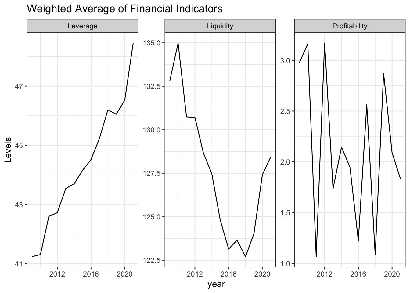

Code

#Calculation and plot of standard deviation of financial indicators
bs_df_economy %>% 
  group_by(year) %>% 
  summarize(Liquidity = sd(current_ratio) * 10,
            Leverage = sd(leverage) * 10,
            Profitability = sd(return_on_assets) * 10) %>% 
  pivot_longer(-year, names_to = "std_yearly", values_to = "value") %>% 
  ggplot(aes(x = year, y = value)) +
  geom_line() +
  facet_wrap(~std_yearly, scales = "free") +
  theme_bw()+
  labs(y = "Levels", title = "Standard Deviation of Financial Indicators")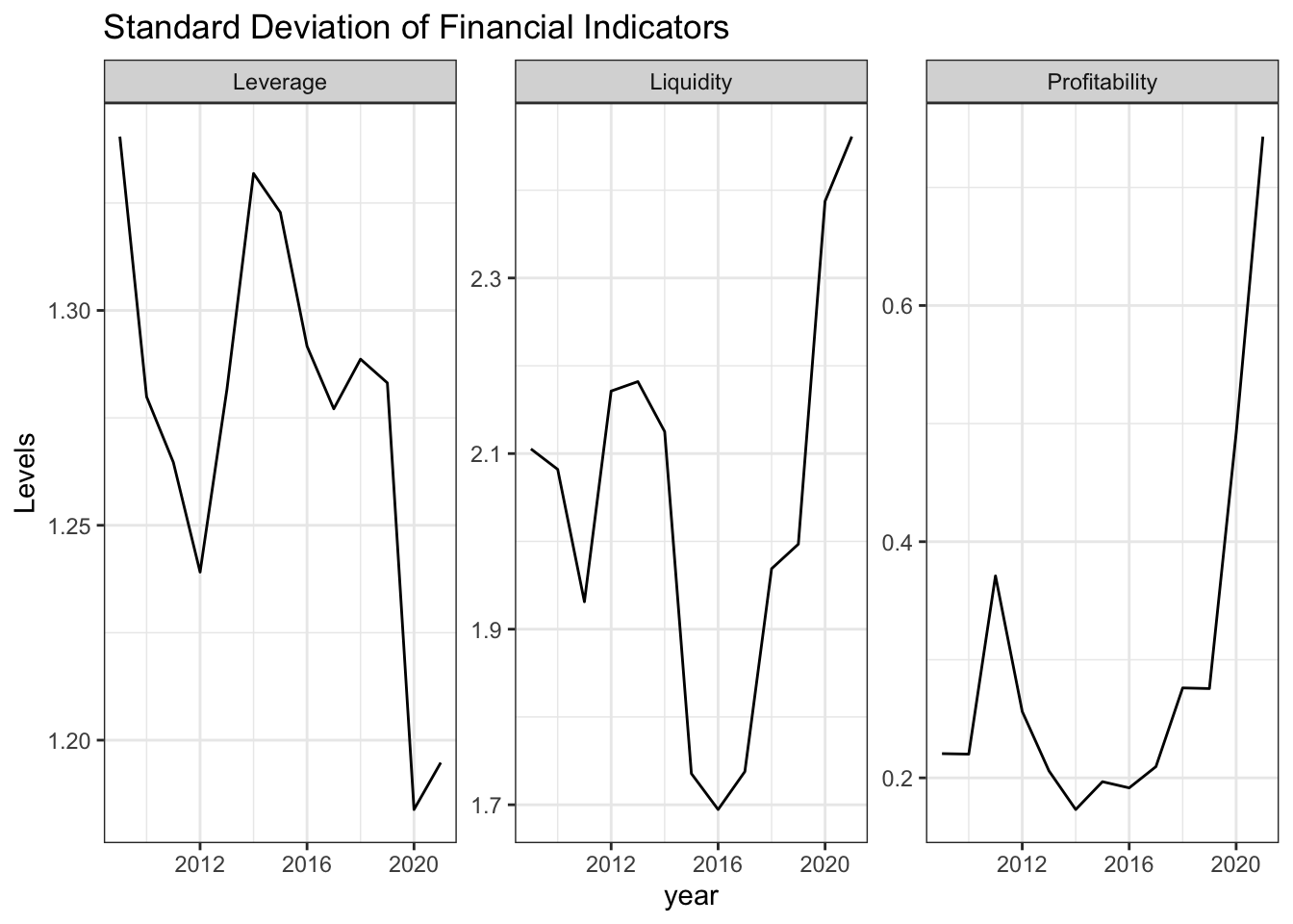

Table of financial indicators for the economy from 2009 to 2021

A table version of the previous plots is given below.

Code

colnames(bs_df_economy_graph) <- c("Year", "Liquidity", "Leverage", "Profitability")
bs_df_economy_graph[,2:4] <- lapply(bs_df_economy_graph[,2:4], 
                                    FUN = function(x) round(x, 2))
kable(bs_df_economy_graph)

Year	Liquidity	Leverage	Profitability
2009	132.77	41.23	2.98
2010	134.97	41.31	3.16
2011	130.74	42.60	1.06
2012	130.70	42.72	3.17
2013	128.67	43.53	1.74
2014	127.47	43.70	2.14
2015	124.81	44.15	1.95
2016	123.14	44.52	1.23
2017	123.65	45.23	2.56
2018	122.70	46.20	1.08
2019	124.03	46.05	2.87
2020	127.41	46.52	2.09
2021	128.45	48.45	1.83

Time Series of Financial Indicators for each sector

Financial indicators are given for each sector below.

Construction, Mining, Information and Manufacturing are the sectors which have an upward trend in their liquidity position and deemed strong in terms of its level as of 2021 as compared to others.

Leverage of real sector firms increased significantly in this period except Construction and Electricity-Gas sectors, which lowers the share of external liabilities in the financing of their assets and can be considered less risky as compared to the beginnning of the period.

In terms of ability to return assets into profits, winner sectors are Manufacturing, Information and Mining where as the harming effect of the COVID-19 is observed in Accomodation-Food, Entertainment and Transportation which is not surprising as these sectors are more dependent on social mobility and the recovery in the period after March-2020 is only gradual. A more benign picture can be observed in 2022 when a complete normalisation in Covid related restrictive policies has been observed. Furthermore, a consistent deterioration in the profits of Construction sector is eye-catching

Code

ggplot(data = bs_df_new[bs_df_new$Indicator == "current_ratio",], aes(x = year, y = Value)) +
  geom_line() +
  labs(title = "Liquidity Indicator of Real Sector Companies from 2009 to 2021", x = "Year") +
  facet_wrap(~sector_name, scales = "free") +
  theme(panel.grid = element_blank()) +
  theme_bw()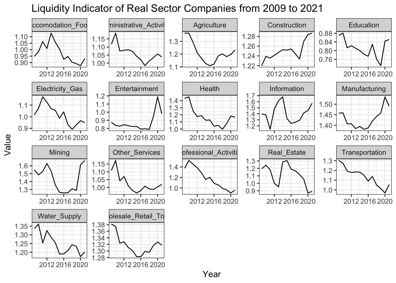

Code

ggplot(data = bs_df_new[bs_df_new$Indicator == "leverage",], aes(x = year, y = Value)) +
  geom_line() +
  labs(title = "Leverage Indicator of Real Sector Companies from 2009 to 2021", x = "Year") +
  facet_wrap(~sector_name, scales = "free") +
  theme(panel.grid = element_blank()) +
  theme_bw()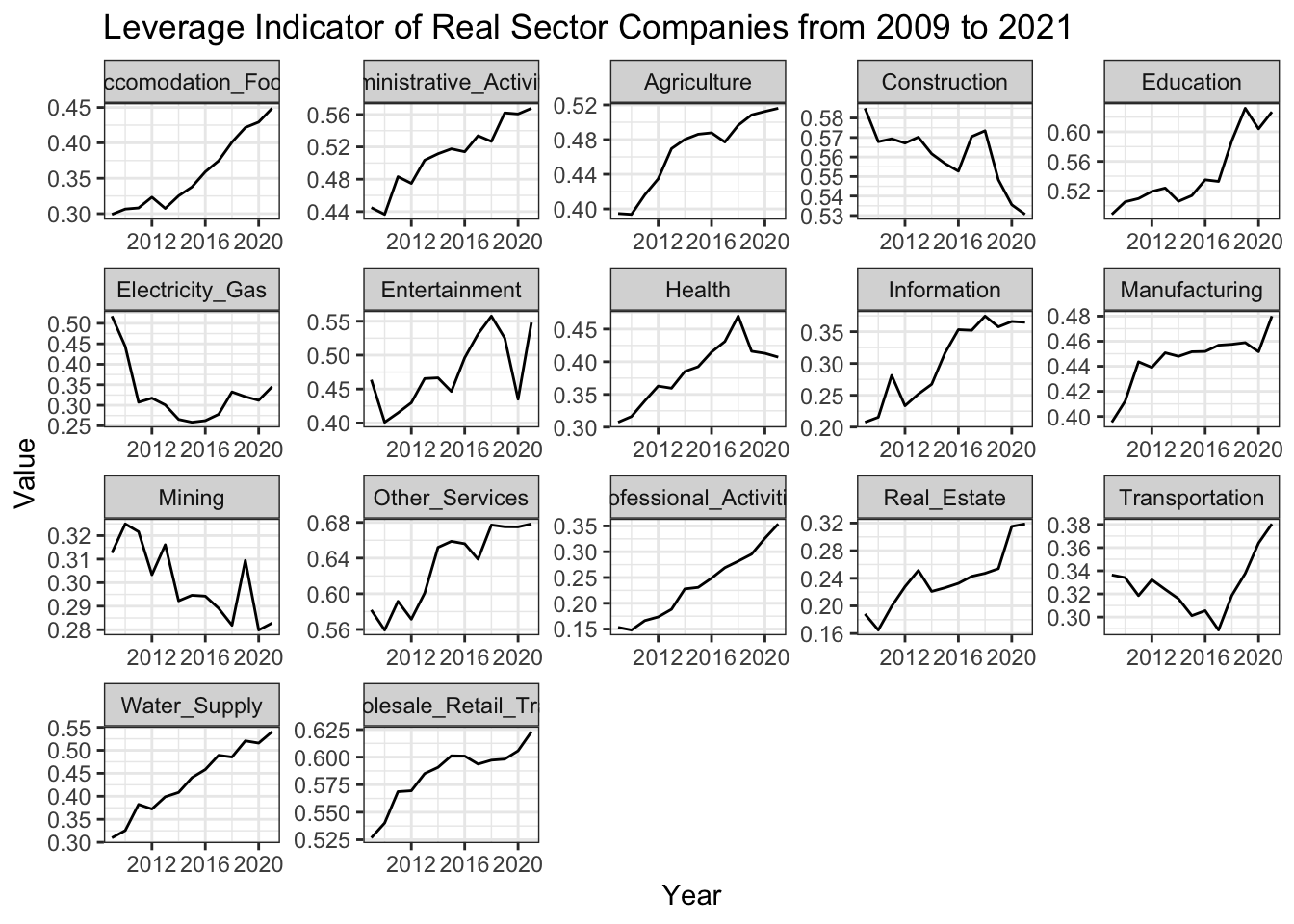

Code

ggplot(data = bs_df_new[bs_df_new$Indicator == "return_on_assets",], aes(x = year, y = Value)) +
  geom_line() +
  labs(title = "Profitability (ROA) Indicator of Real Sector Companies from 2009 to 2021", x = "Year") +
  facet_wrap(~sector_name, scales = "free") +
  theme(panel.grid = element_blank()) +
  theme_bw()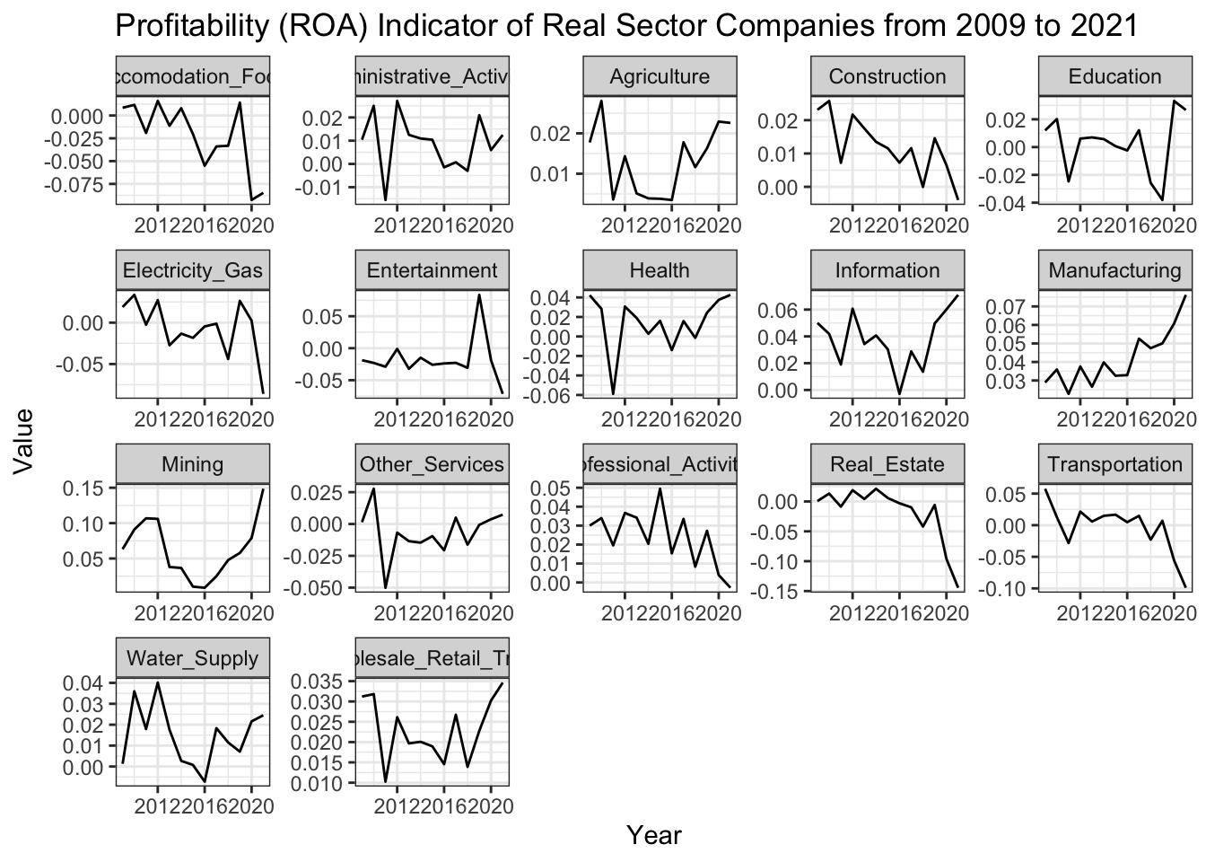

Scatter Plots of Financial Indicators

In the previous section, one dimensional evolution of sectors in time is outlined. Having obtained indicators for financial overview of Turkish Economy on a sectoral basis, temporal relationship between them is worth analysing.

Regarding liquidity and leverage, there exists a clear negative association which is in effect for almost all of the sectors albeit with different degrees.The exception is Mining sector which experiences rise in leverage and liquidity positions at the same time.

For liquidity and profitability, expected outcome is observed such that real sector firms have a better liquidity when they are more profitable for the period in consider.

Lastly, profitability and leverage indicators among sectors demonstrate a trade-off such that in general firms with lower profit encounters a decline in the share of equity as a source of financing.

Code

bs_df_new %>% 
  pivot_wider(names_from = "Indicator", values_from = "Value") %>% 
  ggplot(aes(x = leverage, y = current_ratio, color = sector_name)) +
  geom_point() + 
  geom_smooth(method='lm', formula= y~x, se = FALSE) +
  labs(title = "Liquidity vs Leverage", y = "Liquidity") +
  theme_bw()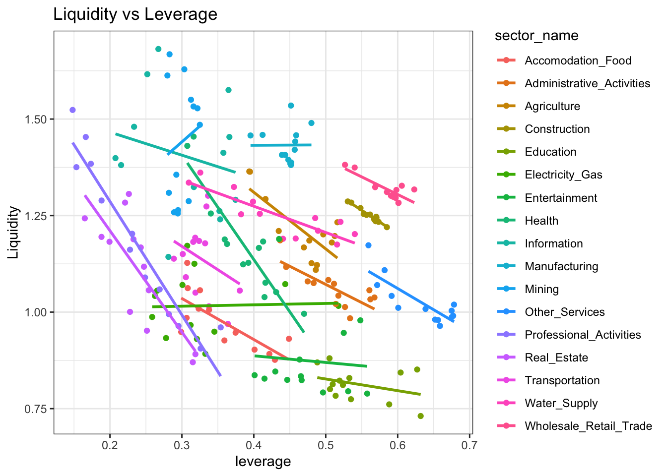

Code

bs_df_new %>% 
  pivot_wider(names_from = "Indicator", values_from = "Value") %>% 
  ggplot(aes(x = current_ratio, y = return_on_assets, color = sector_name)) +
  geom_point() + 
  geom_smooth(method='lm', formula= y~x, se = FALSE) +
  labs(title = "Profitability vs Liquidity", y = "Profitability", x = "Liquidity") +
  theme_bw()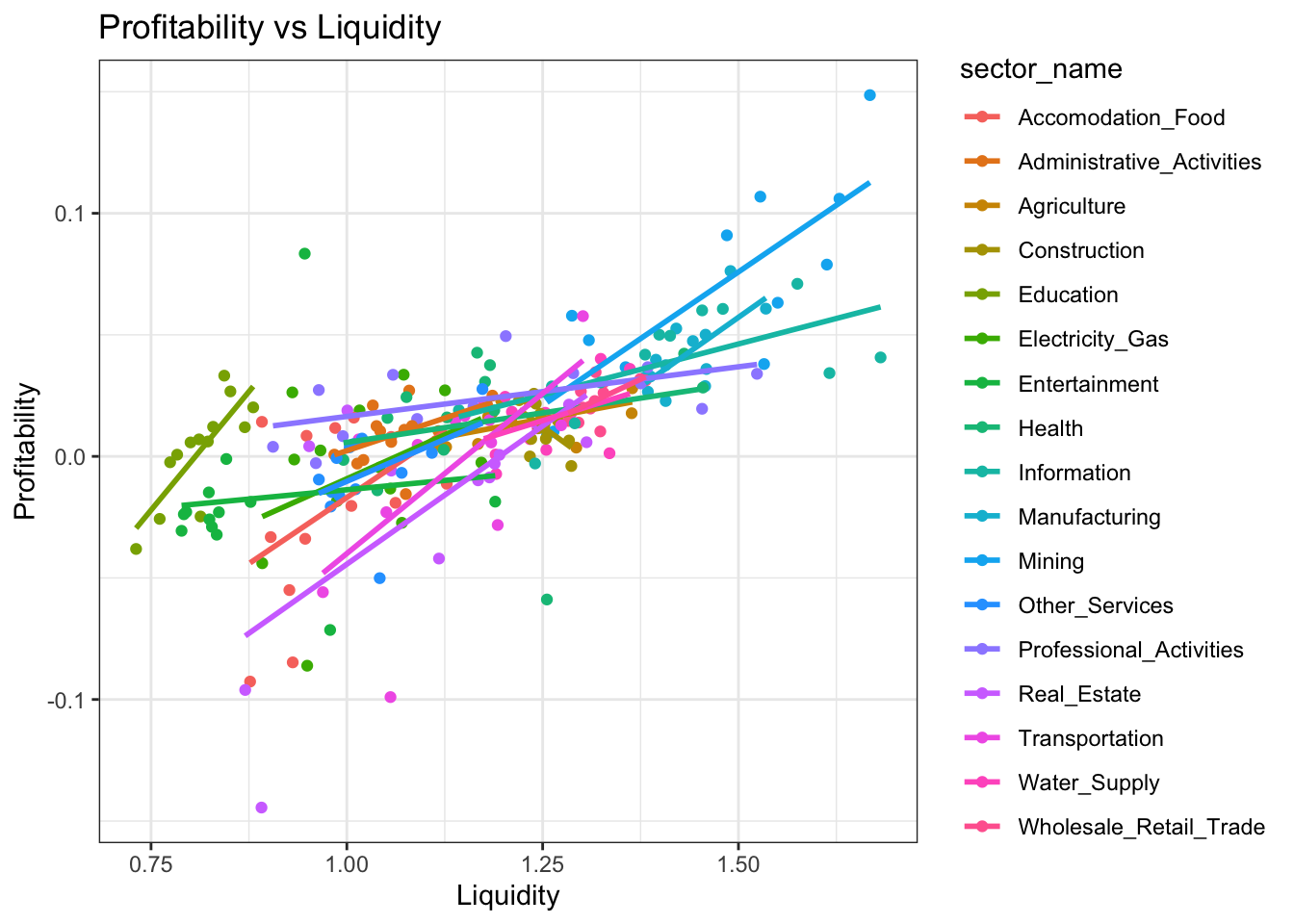

Code

bs_df_new %>% 
  pivot_wider(names_from = "Indicator", values_from = "Value") %>% 
  ggplot(aes(x = leverage, y = return_on_assets, color = sector_name)) +
  geom_point() + 
  geom_smooth(method='lm', formula= y~x, se = FALSE) + 
  labs(title = "Profitability vs Leverage", y = "Profitability") +
  theme_bw()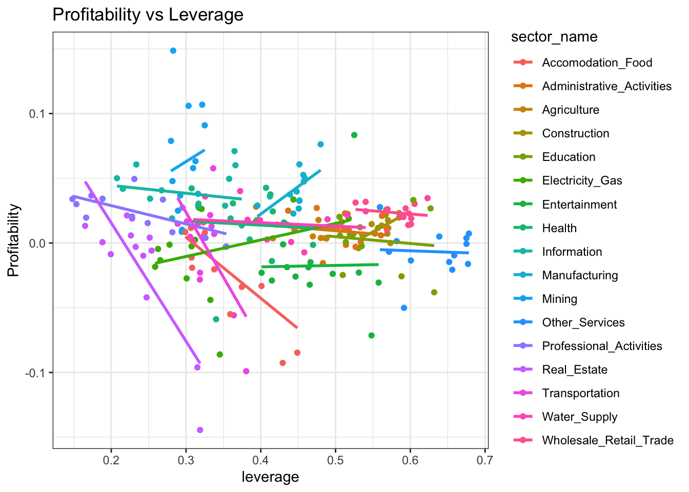

2009 - 2019 Period Average of Financial Indicators

A closer look for the perfomance of Turkish economy in the last two years is aimed to be investigated in comparison to previous years. 2020 and 2021 is important especially for diagnosing the effect of Covid-19 outbreak and its consequent impact on the financial status of real sector firms.

Firstly, Transportation, Accomodation-Food, Real Estate and Professional Activities are the sectors whose liquidity position deteriorate most during Covid-19. This result is not abnormal as social distancing measures and decline in mobility affect those sectors most.The rest seems to be less affected and even there are sectors who experience a considerable improvement in terms of liquidity which might be due to frequency of our data. The covid-19 outbreak started in first quarter of 2020 and then the government policies to support the economy could be one reason for the improvement of the sectors.

Secondly, leverage indicator seemed to rise throughout the economy except a few sectors which is considered natural in response to credit oriented policies of government to support real sector firms against Covid-19 shock.

Finally, the winners are Mining, Manufacturing, Information and Health in terms of improvement in their profits and this improvement seemed to continue in 2021. On the other end of the picture, Transportation and Services sectors were seen to be in trouble in terms of profitability.

Liquidity Indicator

Code

bs_df_average <-  bs_df_new %>% 
  pivot_wider(names_from = Indicator, values_from = Value) %>% 
  filter(year %in% 2009:2019) %>% 
  group_by(sector_name) %>% 
  summarise(liq_ave = mean(current_ratio), lev_ave = mean(leverage), pro_ave = mean(return_on_assets))

bs_df_new %>% 
  pivot_wider(names_from = Indicator, values_from = Value) %>% 
  filter(year %in% 2020:2021) %>% 
  select(c(sector_name, year, current_ratio)) %>% 
  pivot_wider(names_from = year, values_from = current_ratio) %>% 
  left_join(bs_df_average[,c("sector_name", "liq_ave")], by = "sector_name") %>% 
  rename("2009_2019_average" = "liq_ave") %>% 
  pivot_longer(-sector_name, names_to = "period") %>% 
  ggplot(aes(x = sector_name, y = value, fill = factor(period))) +
  geom_col(position = "dodge2")+
  coord_flip() +
  labs(y = "Current Ratio", x = "Sectors", title = "Liquidity Indicator", fill = "Years") +
  theme_bw()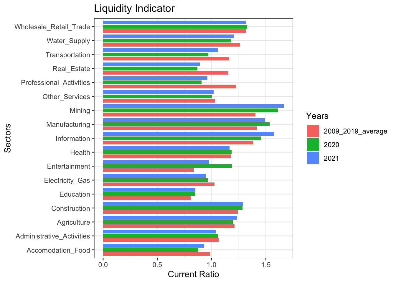

Leverage Indicator

Code

bs_df_new %>% 
  pivot_wider(names_from = Indicator, values_from = Value) %>% 
  filter(year %in% 2020:2021) %>% 
  select(c(sector_name, year, leverage)) %>% 
  pivot_wider(names_from = year, values_from = leverage) %>% 
  left_join(bs_df_average[,c("sector_name", "lev_ave")], by = "sector_name") %>% 
  rename("2009_2019_average" = "lev_ave") %>% 
  pivot_longer(-sector_name, names_to = "period") %>% 
  ggplot(aes(x = sector_name, y = value, fill = factor(period))) +
  geom_col(position = "dodge2")+
  coord_flip() +
  labs(y = "Leverage", x = "Sectors", title = "Leverage Indicator", fill = "Years") + theme_bw()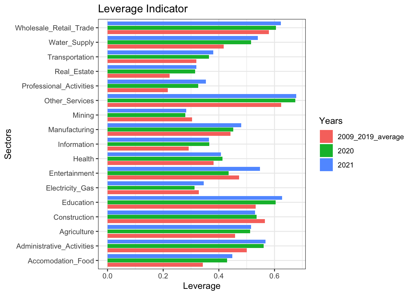

Profitability Indicator

Code

bs_df_new %>% 
  pivot_wider(names_from = Indicator, values_from = Value) %>% 
  filter(year %in% 2020:2021) %>% 
  select(c(sector_name, year, return_on_assets)) %>% 
  pivot_wider(names_from = year, values_from = return_on_assets) %>% 
  left_join(bs_df_average[,c("sector_name", "pro_ave")], by = "sector_name") %>% 
  rename("2009_2019_average" = "pro_ave") %>% 
  pivot_longer(-sector_name, names_to = "period") %>% 
  ggplot(aes(x = sector_name, y = value, fill = factor(period))) +
  geom_col(position = "dodge2")+
  coord_flip() +
  labs(y = "Profitability", x = "Sectors", title = "Return on Assets", fill = "Years") +
  theme_bw()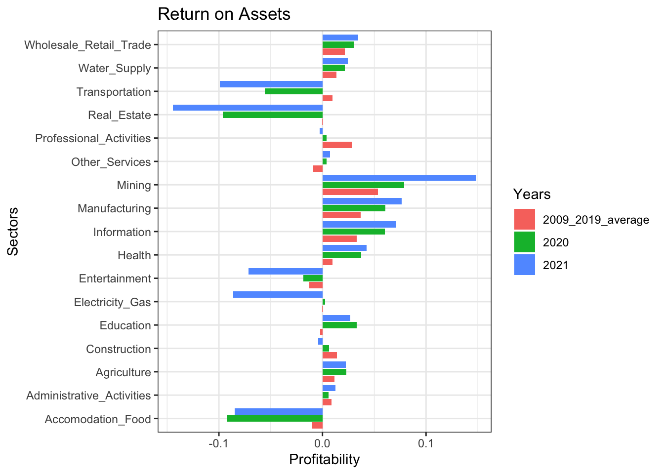

Density Plots of Financial Indicators

Density plots make it possible to observe complete distribution of indicators among sectors in a specific year. In the plots below, distributions are segmented by colors with respect to 25^th, 50^th and 75^th percentiles where white shaded region denotes sectors that are below the 25^th percentile and dark blue region corresponds to sectors above 75^th percentile of the distribution with respect to the financial indicator.

For liquidity, the distribution seems to became right skewed at the end of 2021 vs its left skewed shape back in 2009 which implies that firms’ liquidity position decreases on average while there exists sectors that are in a stronger position in terms of liquidity.

For leverage, aside from increasing median leverage among sectors, no significant change in the shape of the distribution is observed.

For profitability, the obvious picture is that deviation of profitability across sectors increased considerably. Pandemic shock resulted in higher portion of sectors within the economy incurring higher net losses in 2020 as compared to 2019. Although a rebound is expected in profitability of sectors in 2021, distribution presents a different picture where a clear separation between sectors exist such that sectors in loss at the end of 2020 incur higher losses. On the other hand, the gains of some sectors increased comparatively higher in this period and the distribution became flat with outliers in the both end.

Code

# Liquidity
bs_df_new %>% pivot_wider(names_from = Indicator, values_from = Value) %>% 
  select(year, current_ratio) %>% 
  arrange(year) %>% 
  ggplot(aes(x = current_ratio, y = factor(year), fill = stat(quantile))) +
  stat_density_ridges(quantile_lines = FALSE,
                      calc_ecdf = TRUE,
                      geom = "density_ridges_gradient", rel_min_height = 0.005) +
  scale_fill_brewer(name = "") +
  labs(y = "Year", x = "Liquidity")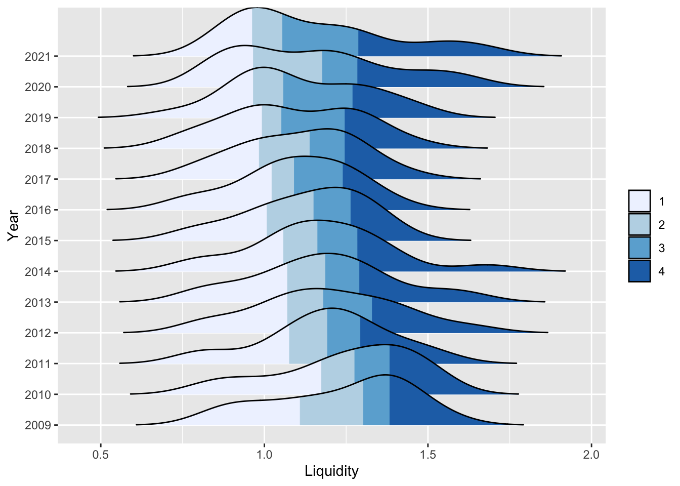

Code

# Leverage
bs_df_new %>% pivot_wider(names_from = Indicator, values_from = Value) %>% 
  select(year, leverage) %>% 
  arrange(year) %>% 
  ggplot(aes(x = leverage, y = factor(year), fill = stat(quantile))) +
  stat_density_ridges(quantile_lines = FALSE,
                      calc_ecdf = TRUE,
                      geom = "density_ridges_gradient", rel_min_height = 0.005) +
  scale_fill_brewer(name = "") +
  labs(y = "Year", x = "Leverage")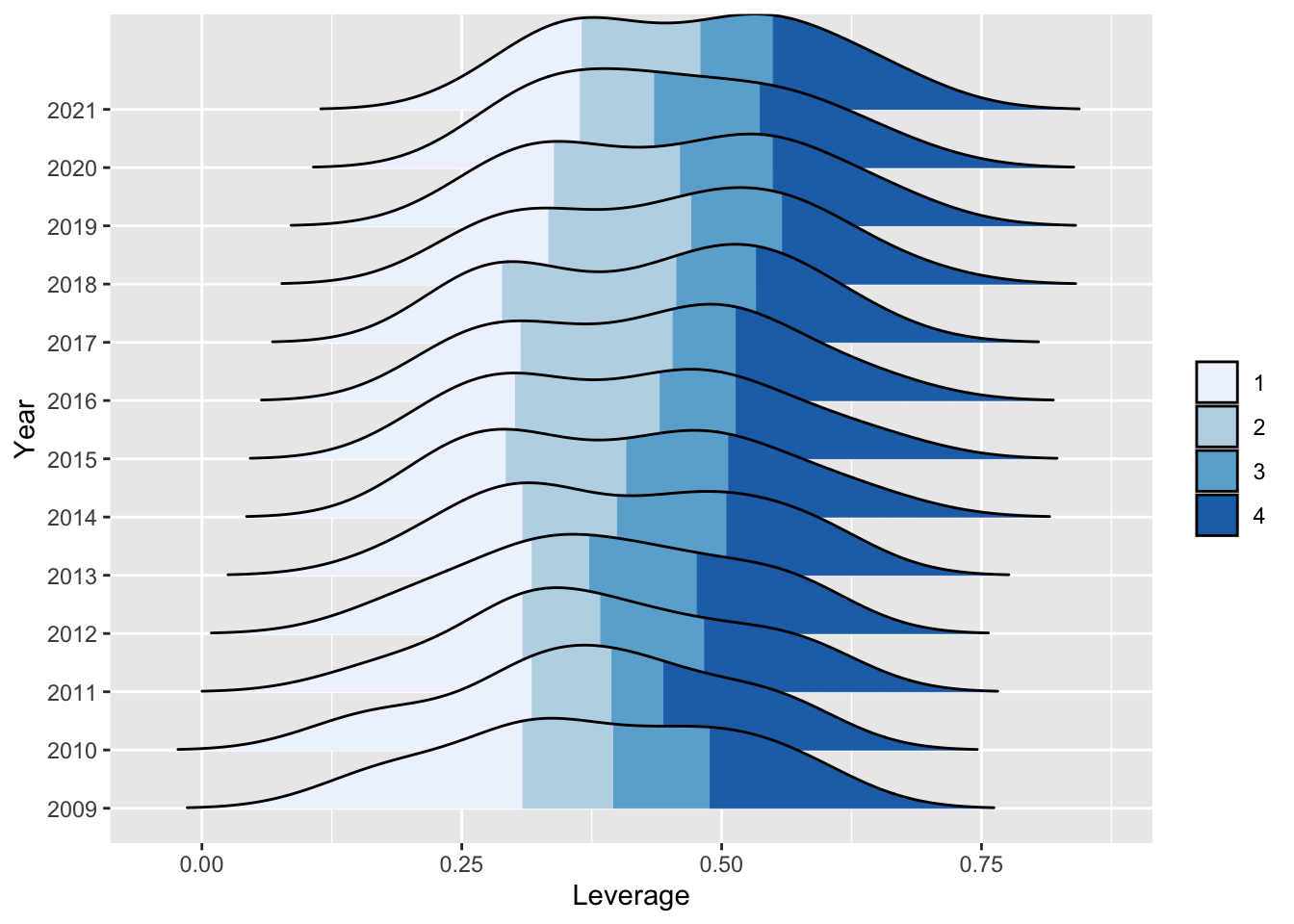

Code

# Profitability
bs_df_new %>% pivot_wider(names_from = Indicator, values_from = Value) %>% 
  select(year, return_on_assets) %>% 
  arrange(year) %>% 
  ggplot(aes(x = return_on_assets, y = factor(year), fill = stat(quantile))) +
  stat_density_ridges(quantile_lines = FALSE,
                      calc_ecdf = TRUE,
                      geom = "density_ridges_gradient", rel_min_height = 0.005) +
  scale_fill_brewer(name = "") + 
  labs(y = "Year", x = "Return on Assets")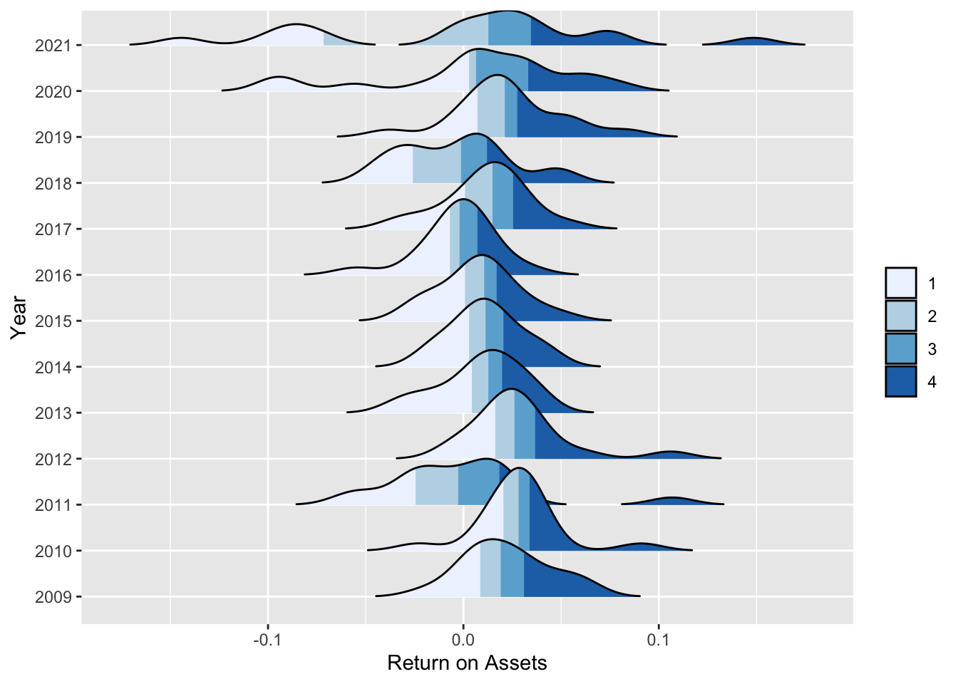

Financial Fragility Index

Up until now, financial position of Turkish economy is evaluated based on the three indicators obtained through balance sheets and income statements of sectors. In this section, an index demonstrating financial healthiness of the sectors is constructed so that a comparative analysis of Turkish economy through time can be conducted on a holistic perspective.

The methodology used in the construction of Financial Fragility Index (FFI) consists of the following steps:

1- For each financial indicator (Liquidity, Leverage and Profitability) percentile of each sector is found. To be more specific, the higher the rank of a sector, the worse it is in terms of financial soundness. In other words, for liquidity, the sector is less liquid, for leverage, the sector has higher leverage and for profitability, the sector is less profitable.

2- After finding each sectors’ rank for each financial indicator, simple average is calculated and index value is obtained.

3- The steps described above is repeated for each year between 2009-2021 and a time series of the index is found.

After obtaining FFI, evolution of the index for each sector is illustrated in the graph below.

Services sectors such as Accomodation-Food, Real Estate and Transportation have performed worse than other sectors and found themselves in a much more fragile position in terms of financial soundness
Although the index alone can not be taken into account alone to conclude that a certain sector is riskier than others financially for a specific time point, time series evolution gives a glimpse of where the sectors are heading into in terms of their financial strength.

Code

bs_df_ffi <- bs_df_new %>% 
  pivot_wider(names_from = "Indicator", values_from = "Value") %>% 
  group_by(year) %>% 
  mutate(liq_rank = percent_rank(current_ratio*-1), 
         lev_rank = percent_rank(leverage), 
         profit_rank = percent_rank(return_on_assets*-1)) %>% 
  mutate(fin_fra_index = (liq_rank + lev_rank + profit_rank)/3) %>% 
  select(-c(current_ratio:return_on_assets))

bs_df_ffi %>% 
  select(c(sector_name, year, fin_fra_index)) %>% 
  pivot_longer(-c(sector_name, year), names_to = "index", values_to = "value") %>% 
  ggplot(aes(x = year, y = value)) +
  geom_line() + 
  facet_wrap(~sector_name, scales = "free") + 
  labs(y = "Financial Fragility Index") +
  theme_bw()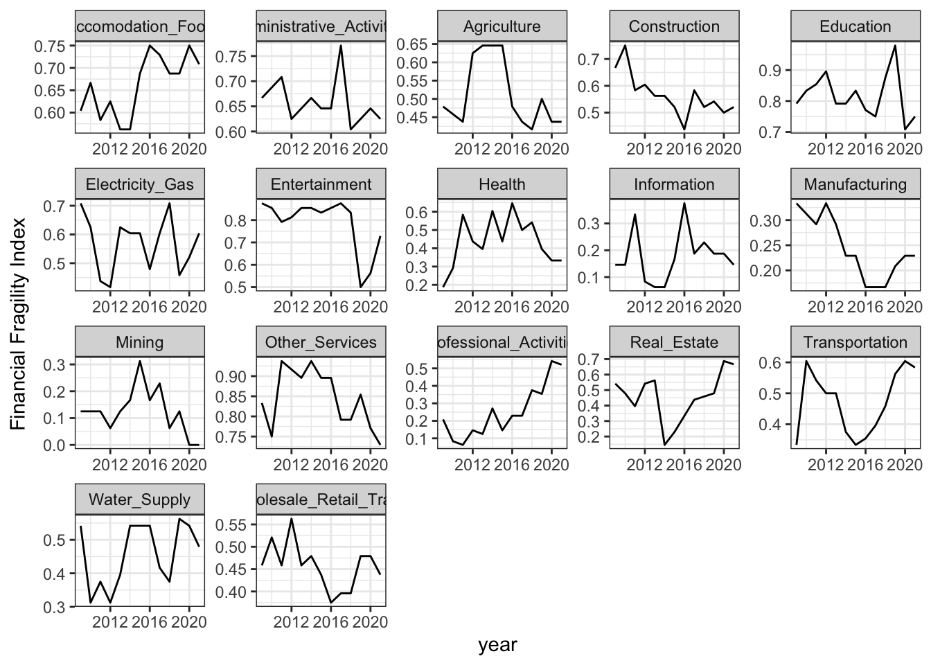

Heatmap for 2021

For 2021, a cross sectional analysis demonstrates that services related sectors are considered most risky in terms of financial metrics defined previously.

Education is considered most risky sector mostly due to its poor liquidity and high leverage which increases the firms’ probability of default as it raises doubts about payment of short term debts.
Mining sector is the leading sector in terms of financial soundness according to all of the predefined metrics.

Code

heatmap_df <- bs_df_economy %>% 
  filter(year == 2021) %>% 
  select(sector_name, current_ratio, leverage, return_on_assets) %>% 
  mutate(ffi = bs_df_ffi %>% select(year, sector_name, fin_fra_index) %>% filter(year == 2021) %>% pull(fin_fra_index)) %>% 
  arrange(desc(ffi)) 

colnames(heatmap_df) <- c("Sectors", "Liquidity", "Leverage", "Profitability", "Financial Fragility Index")

heatmap_df[,2:5] <- lapply(heatmap_df[,2:5], FUN = function(x) round(x*100, 2))

heatmap_df %>% 
  gt() %>% 
  data_color(columns = 'Liquidity', 
             colors = col_numeric(palette = c("red", "white", "green"), 
                                  domain = c(min(heatmap_df[,2]), max(heatmap_df[,2])))) %>% 
  data_color(columns = 'Leverage', 
             colors = col_numeric(palette = c("green", "white", "red"), 
                                  domain = c(min(heatmap_df[,3]), max(heatmap_df[,3])))) %>% 
  data_color(columns = 'Profitability', 
             colors = col_numeric(palette = c("red", "white", "green"), 
                                  domain = c(min(heatmap_df[,4]), max(heatmap_df[,4])))) %>% 
  data_color(columns = 'Financial Fragility Index', 
             colors = col_numeric(palette = c("green", "white", "red"), 
                                  domain = c(min(heatmap_df[,5]), max(heatmap_df[,5]))))

Sectors	Liquidity	Leverage	Profitability	Financial Fragility Index
Education	85.13	62.71	2.67	75.00
Entertainment	97.87	54.81	-7.14	72.92
Other_Services	101.94	67.83	0.73	72.92
Accomodation_Food	93.09	44.88	-8.47	70.83
Real_Estate	89.10	31.88	-14.45	66.67
Administrative_Activities	103.79	56.77	1.25	62.50
Electricity_Gas	94.94	34.52	-8.61	60.42
Transportation	105.57	38.05	-9.90	58.33
Construction	128.66	53.06	-0.40	52.08
Professional_Activities	96.05	35.40	-0.28	52.08
Water_Supply	120.21	54.04	2.45	47.92
Agriculture	123.27	51.61	2.26	43.75
Wholesale_Retail_Trade	131.77	62.30	3.46	43.75
Health	116.63	40.70	4.27	33.33
Manufacturing	148.98	48.01	7.62	22.92
Information	157.52	36.48	7.10	14.58
Mining	166.78	28.28	14.86	0.00

International Trade

The graphs below demonstrate the evolution of yearly net export of each sector (in billion USD). We analysed the relation of sectors’ net exports with their profitability and financial fragility status only for the first four sectors in terms of the size of net imports.

Since the imports of sectors is mainly driven by economic growth performance, it is not surprising to see sectors having stronger financial position in periods with high net imports.

Code

trade_df_new <- 
  trade_df %>% 
  mutate(net_export = (export - import)/1e6) %>% 
  filter(year != 2022) %>% 
  select(sector_name, year, net_export)

df_fin <- bs_df_new %>% pivot_wider(names_from = Indicator, values_from = Value)


trade_df_new %>% 
  ggplot(aes(x = year, y = net_export))+
  geom_line() +
  facet_wrap(~sector_name, scales = "free")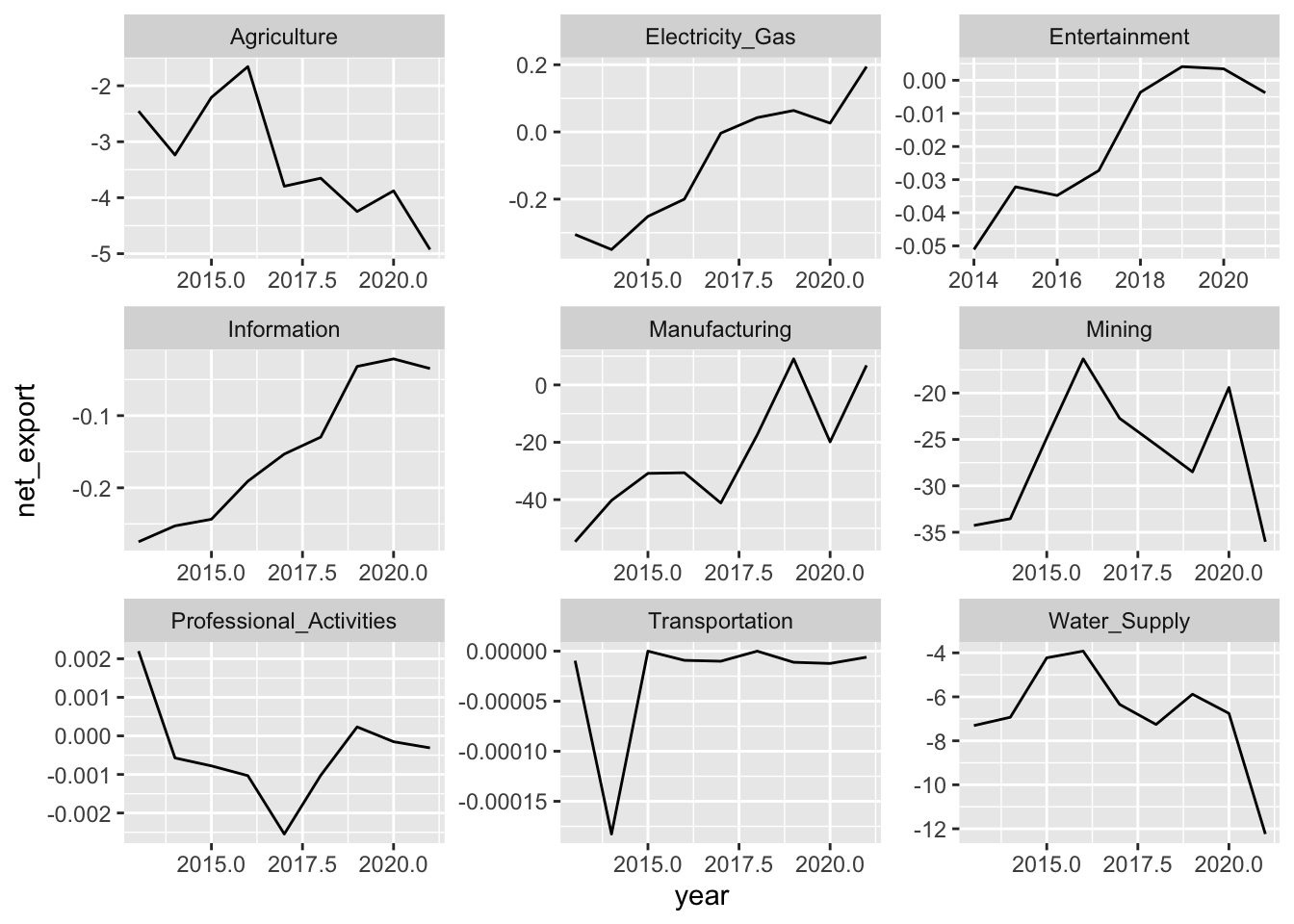

Code

trade_df_new %>% 
  group_by(sector_name) %>% 
  summarize(average = round(mean(net_export), 2)) %>% 
  arrange(average) %>% 
  kable(caption = "Average Net Exports")

Average Net Exports
sector_name	average
Mining	-26.80
Manufacturing	-24.33
Water_Supply	-6.76
Agriculture	-3.34
Information	-0.15
Electricity_Gas	-0.09
Entertainment	-0.02
Professional_Activities	0.00
Transportation	0.00

Code

trade_df_new %>% 
  filter(sector_name %in% c("Agriculture", "Manufacturing", "Mining", "Water_Supply")) %>% 
  inner_join(df_fin %>% select(-sector_code, -group), by = c("sector_name", "year")) %>% 
  ggplot(aes(x = net_export, y = return_on_assets))+
  geom_point() + 
  geom_smooth(method='lm', formula= y~x, se = FALSE) + 
  facet_wrap(~sector_name, scales = "free")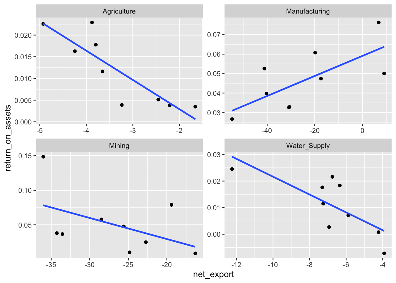

Code

trade_df_new %>% 
  filter(sector_name %in% c("Agriculture", "Manufacturing", "Mining", "Water_Supply")) %>% 
  inner_join(df_fin %>% select(-sector_code, -group), by = c("sector_name", "year")) %>% inner_join(bs_df_ffi %>% select(sector_name, year, fin_fra_index), by = c("sector_name", "year")) %>% 
  ggplot(aes(x = net_export, y = fin_fra_index))+
  geom_point() + 
  geom_smooth(method='lm', formula= y~x) + 
  facet_wrap(~sector_name, scales = "free")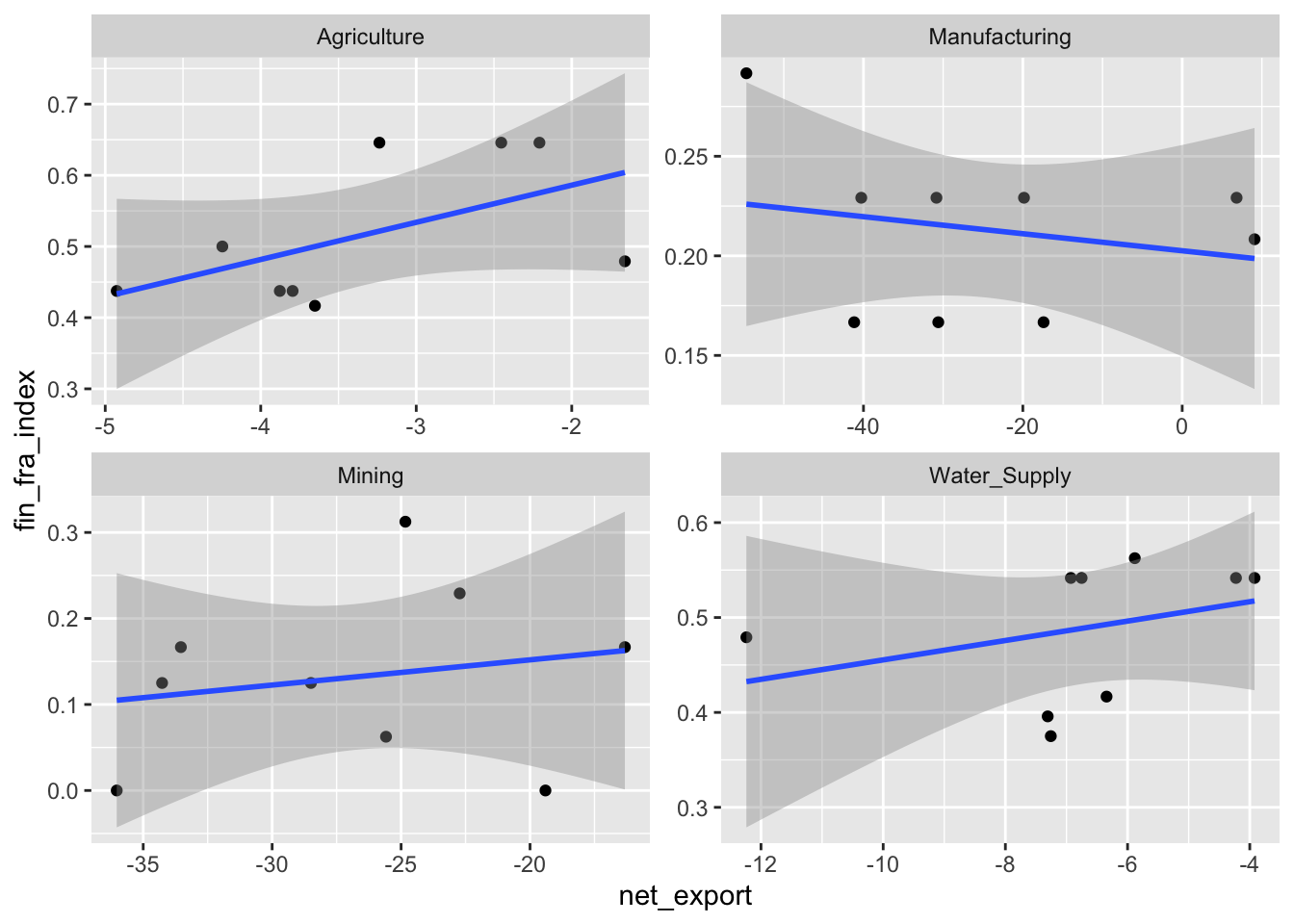

Tradable vs Non-Tradable Sectors

Code

tradables <- c("Agriculture", "Manufacturing", "Mining", "Water_Supply")

df_fin <- df_fin %>% inner_join(bs_df_ffi %>% select(sector_name, year, fin_fra_index), by = c("sector_name", "year"))

df_fin %>% 
  select(-sector_code, -group) %>% 
  mutate(trade_group = ifelse(sector_name %in% tradables, "tradable", "non_tradable")) %>% 
  group_by(year, trade_group) %>% 
  summarize(financial_fragility_index = mean(fin_fra_index)) %>% 
  ggplot(aes(year, financial_fragility_index, color = trade_group)) + 
  geom_line()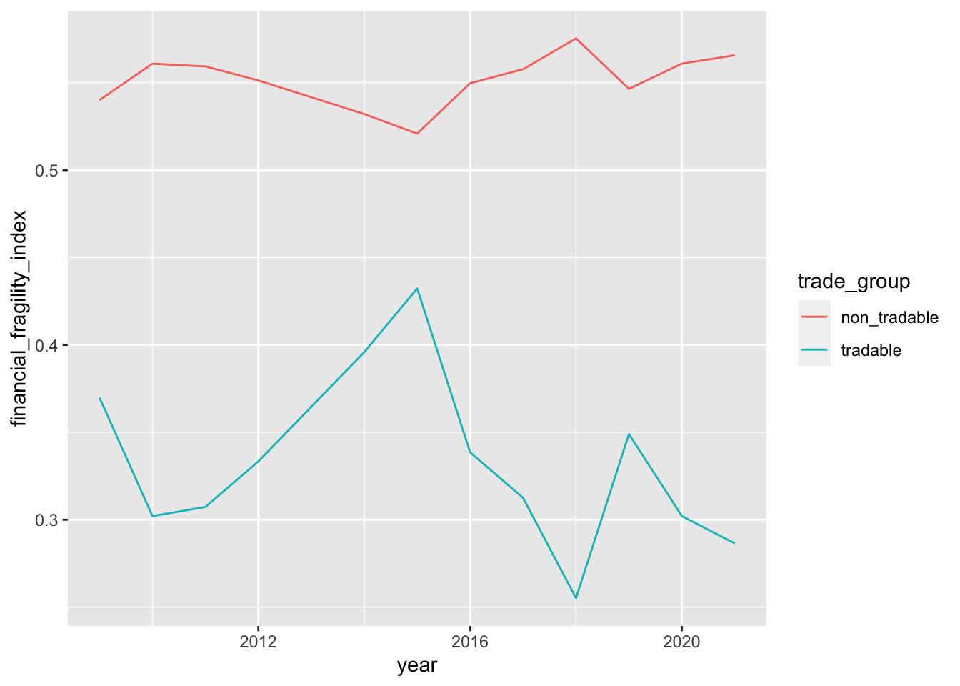

Growth Dynamics

Growth dynamics of the country is an important determinant of country’s financial performance as yearly GDP growth measures the performance of the country’s economy in terms of goods and services produced in that year. Since 2009, highest average growth is achieved by Financial and insurance activities where as the lowest average growth is achieved by Agriculture, forestry and fishing sectors.

Code

gdp_df$pct_change <- (gdp_df$gdp_index / lag(gdp_df$gdp_index, 1) - 1) * 100

gdp_df <- gdp_df %>% filter(!is.na(pct_change) & year >= 2009)

# Real GDP Growth Summary Table 

gdp_df_tb <- gdp_df

setDT(gdp_df)
gdp_df[, as.list(summary(pct_change)), by = sector]

                                                                            sector
 1:                                                                          Total
 2:                                           A- Agriculture, forestry and fishing
 3:                                                                 BCDE- Industry
 4:                                                               C- Manufacturing
 5:                                                                F- Construction
 6:                                                                  GHI- Services
 7:                                               J- Information and communication
 8:                                          K- Financial and insurance activities
 9:                                                      L- Real estate activities
10:                MN- Professional, administrative and support service activities
11: OPQ- Public administration, education, human health and social work activities
12:                                                  RST- Other service activities
           Min.    1st Qu.   Median     Mean   3rd Qu.      Max.
 1:  -4.8395779  3.0774892 4.886660 5.160433  8.592330 11.602185
 2:  -2.9425309  2.1253483 3.300360 3.089001  4.919164  9.256697
 3:  -8.4482154  3.0346335 5.013533 5.891598  9.686020 17.412060
 4:  -8.6292531  2.0623298 5.608743 6.006734  9.541860 19.967008
 5: -15.9068747 -1.8675766 4.948874 4.295708  9.372647 24.878645
 6: -10.2595397  1.2391890 6.406098 5.480158  8.243056 21.342332
 7:  -2.1329458  5.0496912 6.798608 7.824746  9.225318 21.950574
 8:  -6.2618952  3.0949580 7.524540 9.466583 10.227967 30.157813
 9:  -0.1600322  2.3612458 2.792944 2.943916  3.599191  4.933052
10:  -5.1717142 -0.1843973 8.222537 6.748606 12.052047 16.967597
11:   1.2629144  2.9946977 4.645327 4.531002  5.360318 10.147852
12:  -0.3814016  4.2987391 5.805904 7.307440  8.562325 24.807844

Code

gdp_df_tb$sector <- gdp_df_tb %>% 
  select(-gdp_index) %>% .$sector %>% gsub("-.*", "", .)


bs_df_new <- bs_df_new %>% pivot_wider(names_from = Indicator, values_from = Value) %>% 
  left_join(bs_df_ffi %>% select(sector_code, year, fin_fra_index), by = c("sector_code", "year")) %>% 
  pivot_longer(-c(sector_code : year), names_to = "Indicator", values_to = "Value")

fin_ind_group <- bs_df_new %>% 
  select(sector_code, year, Indicator, Value) %>% 
  mutate(group = case_when(sector_code == "A" ~ "A", 
            sector_code %in% c("B", "C", "D", "E") ~ "BCDE", 
            sector_code == "F" ~ "F",
            sector_code %in% c("G", "H", "I") ~ "GHI",
            sector_code == "J" ~ "J",
            sector_code == "L" ~ "L",
            sector_code %in% c("M", "N") ~ "MN",
            TRUE ~ "other")) %>% 
  filter(group != "other") %>% 
  left_join(bs_df %>% select(sector_code, year, Total_assets), Total_assets, by = c("sector_code", "year")) %>%
  select(-sector_code) %>% 
  group_by(group, year, Indicator) %>% 
  summarise(value = weighted.mean(Value, Total_assets)) %>% pivot_wider(names_from = Indicator, values_from = value)

header <- c("A", "BCDE", "F", "GHI", "J", "L", "MN")
names <- c("Agriculture", "Industry", "Construction", "Services", "Information", "Real Estate", "Other Services")
growth_info <- data.frame(header, names)

growth_df <- left_join(fin_ind_group, gdp_df_tb %>% select(-gdp_index),by = c("group" = "sector", "year"))
growth_df <- growth_df %>% 
  left_join(growth_info, by = c("group" = "header"))

growth_df %>% 
  ggplot(aes(lag(pct_change,1), fin_fra_index)) +
  geom_point() + 
  facet_wrap(~names,  scales = "free") + 
  geom_smooth(method='lm', formula= y~x, se = FALSE)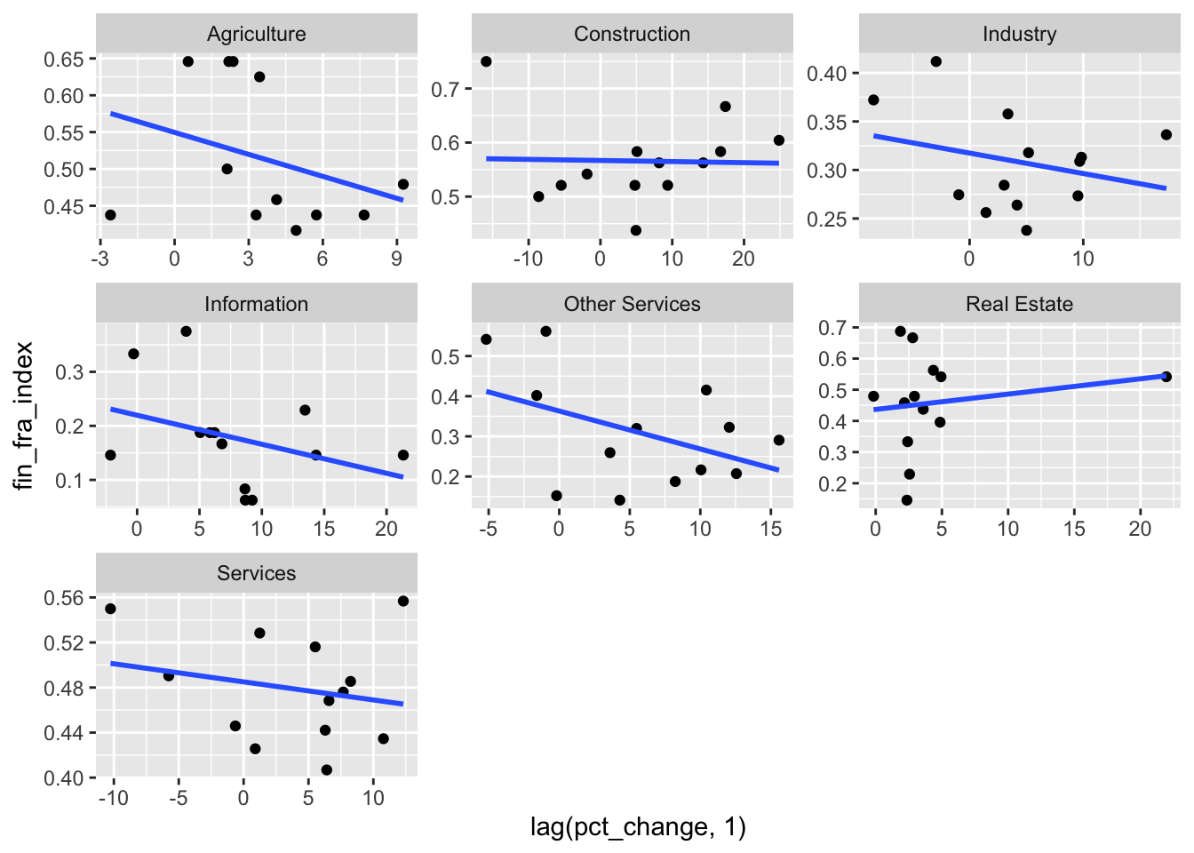

Sectoral Gender Distribution

Code

#Gender distribution in main sectors that are agriculture, construction, industry and services.
emp_data <- readRDS("docs/Project_Data/employment.rds")

table <- emp_data %>%
  group_by(group, gender) %>%
  arrange(sector_name) %>%
  mutate("value") %>%
  summarise(value=sum(number))

table

# A tibble: 8 × 3
# Groups:   group [4]
  group        gender  value
  <chr>        <chr>   <dbl>
1 Agriculture  female 14311 
2 Agriculture  male   20094 
3 Construction female   616 
4 Construction male   11822 
5 Industry     female 11093 
6 Industry     male   33554 
7 Services     female 34383.
8 Services     male   60572.

Code

ggplot(table, aes(x=group, y=value, fill=gender)) +
    geom_bar(stat='identity', position='dodge')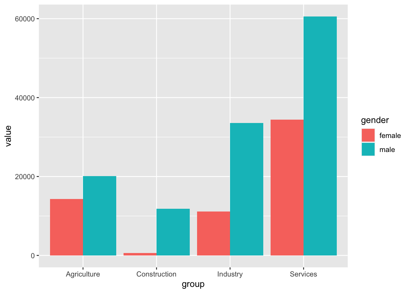

Code

#Detailed gender distribution
emp_data <- readRDS("docs/Project_Data/employment.rds")

table_2 <- emp_data %>%
  group_by(sector_name, gender) %>%
  arrange(sector_name) %>%
  mutate("value") %>%
  summarise(value=sum(number))

ggplot(table_2, aes(x=sector_name, y=value, fill=gender)) +
    geom_bar(stat='identity', position='dodge') + 
    theme(axis.text.x = element_text(angle=90, hjust=1))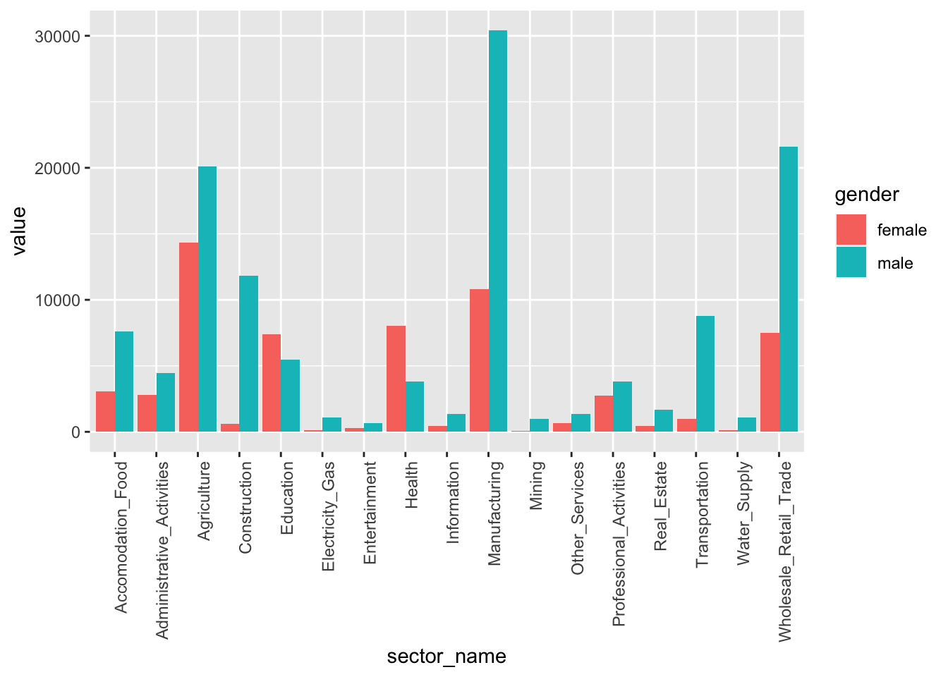

Code

#Percentage of the number of employees in the sectors
emp_data <- readRDS("docs/Project_Data/employment.rds")

table_3 <- emp_data %>%
  group_by(sector_name) %>%
  arrange(sector_name) %>%
  mutate("value") %>%
  summarise(value=sum(number))

total = sum(table_3$value)

table_4 <- table_3 %>%
  group_by(sector_name) %>%
  arrange(sector_name) %>%
  mutate("percentage") %>%
  summarise(percentage=100*value/total)

table_4

# A tibble: 17 × 2
   sector_name               percentage
   <chr>                          <dbl>
 1 Accomodation_Food              5.73 
 2 Administrative_Activities      3.89 
 3 Agriculture                   18.5  
 4 Construction                   6.67 
 5 Education                      6.90 
 6 Electricity_Gas                0.640
 7 Entertainment                  0.504
 8 Health                         6.37 
 9 Information                    0.970
10 Manufacturing                 22.1  
11 Mining                         0.570
12 Other_Services                 1.10 
13 Professional_Activities        3.49 
14 Real_Estate                    1.14 
15 Transportation                 5.24 
16 Water_Supply                   0.640
17 Wholesale_Retail_Trade        15.6

Firm Size Comparison by Sector Groups

Code

#Firm size comparison in the sectors; agriculture, construction, industry and services.
options(dplyr.summarise.inform = FALSE)
sectorinf_data <- readRDS("docs/Project_Data/sector_information.rds")

table_sectorinf <- sectorinf_data %>%
  filter(number == 'Number_of_companies') %>%
  filter(size != 'Total') %>%
  group_by(group,size) %>%
  mutate("num_of_companies") %>%
  summarise(num_of_companies=sum(value)) %>%
  arrange(group,desc(size))

table_sectorinf

# A tibble: 16 × 3
# Groups:   group [4]
   group        size   num_of_companies
   <chr>        <chr>             <dbl>
 1 Agriculture  Small             18265
 2 Agriculture  Micro             94969
 3 Agriculture  Medium             3398
 4 Agriculture  Large               489
 5 Construction Small            307612
 6 Construction Micro            982200
 7 Construction Medium            58513
 8 Construction Large              8144
 9 Industry     Small            471473
10 Industry     Micro            995452
11 Industry     Medium           152032
12 Industry     Large             45049
13 Services     Small           1255079
14 Services     Micro           4300865
15 Services     Medium           260793
16 Services     Large             55289

Code

table_sectorinf %>%
  ggplot(aes(x=group,y=num_of_companies, fill=size)) + 
  geom_bar(stat='identity', position='dodge') +
  xlab("Number of companies") +
  ylab("Sector group")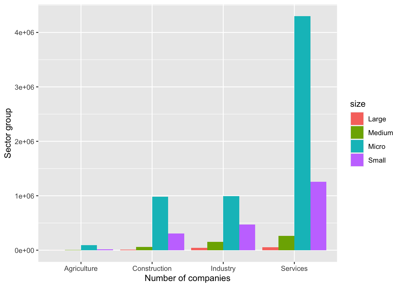

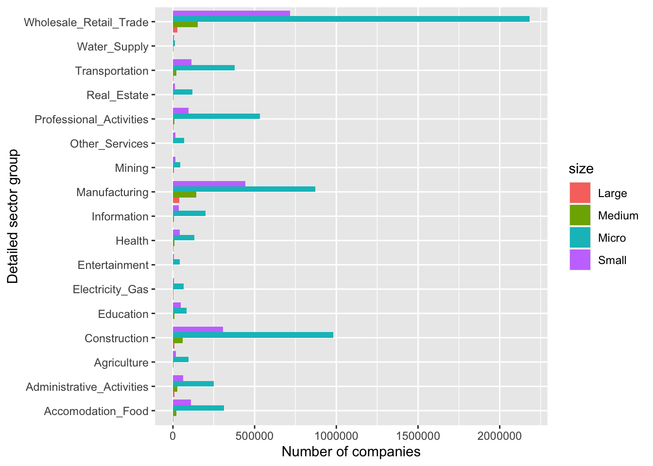
Code

#Firm size comparison by sector names as a detailed version.
table_sectordetail <- sectorinf_data %>%
  filter(number == 'Number_of_companies') %>%
  filter(size != 'Total') %>%
  group_by(sector_name, size) %>%
  mutate("num_of_companies") %>%
  summarise(num_of_companies=sum(value)) %>%
  arrange(sector_name,desc(size))

table_sectordetail

# A tibble: 68 × 3
# Groups:   sector_name [17]
   sector_name               size   num_of_companies
   <chr>                     <chr>             <dbl>
 1 Accomodation_Food         Small            109977
 2 Accomodation_Food         Micro            313604
 3 Accomodation_Food         Medium            20495
 4 Accomodation_Food         Large              3995
 5 Administrative_Activities Small             63121
 6 Administrative_Activities Micro            248544
 7 Administrative_Activities Medium            27225
 8 Administrative_Activities Large             10489
 9 Agriculture               Small             18265
10 Agriculture               Micro             94969
# … with 58 more rows

Code

table_sectordetail %>%
  ggplot(aes(y=sector_name,x=num_of_companies, fill=size)) + 
  geom_bar(stat='identity', position='dodge') +
  xlab("Number of companies") +
  ylab("Detailed sector group")