Agriculture in Turkey - EDA is the part 2 of the Group Project: Agriculture in Turkey
KEY TAKEAWAYS
Key takeaways of the report as follows;
According to TUIK agricultural area datas, Konya, Ankara and Şanlıurfa are top 3 cities having greatest agricultural areas. Konya alone has %8 of agricultural areas of Turkey. Kilis has the most dense agricultural area, comparing to its total area, %71 of the city is agricultural.
In Turkey, 9.213.278 decare (9213,28 km2) agricultural areas is lost in last 12 years, first improvement since 2011 was in 2020, “the pandemic year” but in general in 12 years, size of the agricultural areas moving downwards.
Eastern part of the Turkey loss agricultural land at the highest rate in the first years of decade, “Büyüksehir Yasası” that enacted in the 2012 can be cause of this situation
Yearly Grain/Fruit/Vegetable Production Areas is examined; we find that, increase in the agricultural areas after 2019 due to fruit (mostly nuts) and grain production.
Increase in average temperature in Turkey in 2018, also coincides with the decrease in Agricultural area in that year. We could not observe a clear relation between CO2 emission and agricultural area loss in Turkey. We find out that there is a complex relationship between agricultural loss and CO2 emissions.
We start by loading our dataset that we prepare in the Group Project: Agriculture in Turkey - Preprocessing
Call necessary libraries
#install.packages("readxl")
#install.packages("ggrepel")
#install.packages("plotly")
library(plotly)
library(readxl)
library(lubridate)
library(dplyr)
library(tidyverse)
library(ggplot2)
library(tidyr)
library(ggrepel)
Load the Data
# Prepare data
tarim <- readRDS("data//tarim.rds")
meyve <- readRDS("data//meyve.rds")
sebze <- readRDS("data//sebze.rds")
tahil <- readRDS("data//tahil.rds")
regions <- readRDS("data//Regions.rds")
turkey <- readRDS("data//turkey.rds")
Total Agriculture Areas
total_2021_area <- tarim %>%
  filter(year==2021)%>%
  group_by(year)%>%
  summarise(TotalArea=sum(decare))

Total_Agricultural_Area <- total_2021_area$TotalArea


df_province <- tarim %>%
  filter(year==2021)%>%
  group_by(province_code,province) %>%
  summarise(Agricultural_Area=sum(decare),Total_Agricultural_Area,AgrRatetoTotalAgr=round(Agricultural_Area/Total_Agricultural_Area,2))%>%
  arrange(desc(AgrRatetoTotalAgr))

knitr::kable(head(df_province,10),caption = "Total Agricultural Areas (in Decare) in Turkey 2021 - Top 10 Province")| province_code | province | Agricultural_Area | Total_Agricultural_Area | AgrRatetoTotalAgr |
|---|---|---|---|---|
| 42 | Konya | 18710259 | 234728774 | 0.08 |
| 6 | Ankara | 11639638 | 234728774 | 0.05 |
| 63 | Şanlıurfa | 10445551 | 234728774 | 0.04 |
| 58 | Sivas | 7817565 | 234728774 | 0.03 |
| 66 | Yozgat | 6203771 | 234728774 | 0.03 |
| 1 | Adana | 4871854 | 234728774 | 0.02 |
| 10 | Balıkesir | 3911237 | 234728774 | 0.02 |
| 19 | Çorum | 5415198 | 234728774 | 0.02 |
| 20 | Denizli | 3574561 | 234728774 | 0.02 |
| 21 | Diyarbakır | 5735761 | 234728774 | 0.02 |
Density of Agriculture Areas
To find how dense are the cities in terms of agriculture, we must find total areas of each cities, I used Wikipedia as a data source, First 5 columns are from Wikipedia, geographic locations of each city is taken with geopy library pf Pyhton, and also it’s important to mention that Area is in km2.
head(turkey)# A tibble: 6 × 7
Code Name Area `Population (2000 census)` Popul…¹ Latit…² Longi…³
<chr> <chr> <dbl> <dbl> <dbl> <dbl> <dbl>
1 1 Adana 14046. 1854270 2237940 37.0 35.3
2 2 Adıyaman 7606. 623811 626465 37.8 38.3
3 3 Afyonkarahisar 14719. 812416 729483 38.7 30.6
4 4 Ağrı 11499. 528744 536199 39.8 43.2
5 5 Amasya 5704. 365231 337800 40.7 35.8
6 6 Ankara 25402. 4007860 5639076 39.9 32.9
# … with abbreviated variable names ¹`Population (2019-2020 estimate)`,
# ²Latitude, ³LongitudeJoin the turkey dataframe with turkey_tarim_area_21, Area is in km2 and Total_Province_Area is in Decare,
turkey_tarim_area_21 = merge(turkey, df_province, by.x = 'Code', by.y = 'province_code')
head(turkey_tarim_area_21)
Code Name Area Population (2000 census)
1 1 Adana 14045.56 1854270
2 10 Balıkesir 14472.73 1076347
3 11 Bilecik 4306.77 194326
4 12 Bingöl 8253.51 253739
5 13 Bitlis 7094.50 388678
6 14 Bolu 8323.39 270654
Population (2019-2020 estimate) Latitude Longitude province
1 2237940 36.98636 35.32529 Adana
2 1228650 39.54008 28.02288 Balıkesir
3 219427 40.14351 29.97529 Bilecik
4 279812 39.07380 40.72962 Bingöl
5 348115 38.49509 42.16784 Bitlis
6 316126 40.62121 31.64603 Bolu
Agricultural_Area Total_Agricultural_Area AgrRatetoTotalAgr
1 4871854 234728774 0.02
2 3911237 234728774 0.02
3 838109 234728774 0.00
4 294903 234728774 0.00
5 1388963 234728774 0.01
6 1139150 234728774 0.00Kilis is the most dense city in terms of agricultural areas,
df_area_to_ag <- turkey_tarim_area_21 %>%
  group_by(province) %>%
  summarise(Agricultural_Area,Density = Agricultural_Area*0.001/Area ) %>%
  arrange(desc(Density))

knitr::kable(head(df_area_to_ag,10),caption = "Density of Agricultural Areas (Agricultural Area/Area) in 2021 - Top 10 Province")| province | Agricultural_Area | Density |
|---|---|---|
| Kilis | 1017790 | 0.7128579 |
| Kırıkkale | 3082717 | 0.6745906 |
| Tekirdağ | 4154336 | 0.6550204 |
| Nevşehir | 3303465 | 0.6127013 |
| Edirne | 3306122 | 0.5421730 |
| Şanlıurfa | 10445551 | 0.5402067 |
| Gaziantep | 3466184 | 0.5063937 |
| Kırşehir | 3265004 | 0.4999761 |
| Aksaray | 3843131 | 0.4824714 |
| Konya | 18710259 | 0.4584329 |
Now, lets plot the agricultural areas of Turkish cities in 2021, both size corresponds to total agricultural areas in 2021 and color corresponds to density of Agricultural Areas.
# Plot the Turkey province data
# Extract the data we're interested in
ggplot(data = turkey_tarim_area_21) +
  geom_point(aes(x = Longitude, y =Latitude ,
                 color = -log10((Agricultural_Area*0.001/Area)*100),
                 size = Agricultural_Area,
                 label = Name), alpha = 0.6) +
  scale_size(name = "Agricultural Area",
             range = c(5, 15)) +
  theme(legend.position = "up") +
  labs(x = "longitude",
       y = "latitude",
       title = "Turkey: Agricultural Areas") +
geom_text(aes(x =Longitude , y = Latitude, label = Name)) 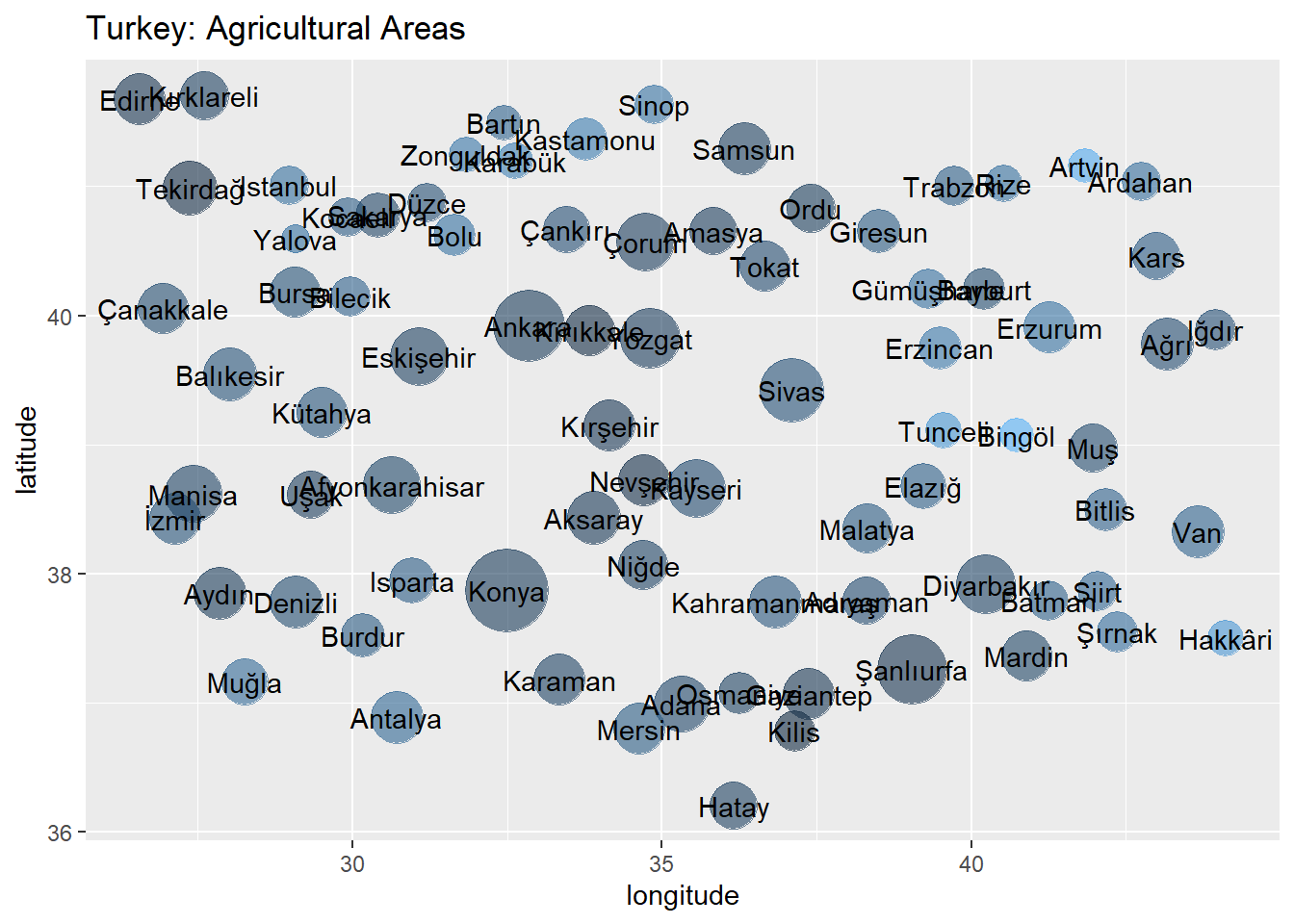
Agriculture areas are shrinking slightly
df <- tarim %>%
  group_by(year) %>%
  summarise(TotalAgricultureDecare=sum(decare)) %>%
  arrange(year) %>%
  mutate(prev=lag(TotalAgricultureDecare)) %>%
  mutate(diff =TotalAgricultureDecare-prev ) %>%
  mutate(totalloss= sum(diff, na.rm=TRUE))

df
# A tibble: 12 × 5
year TotalAgricultureDecare prev diff totalloss
<dbl> <dbl> <dbl> <dbl> <dbl>
1 2010 243942052 NA NA -9213278.
2 2011 236137614. 243942052 -7804438. -9213278.
3 2012 237819993. 236137614. 1682379. -9213278.
4 2013 238055119. 237819993. 235126. -9213278.
5 2014 239407138. 238055119. 1352018. -9213278.
6 2015 239336141. 239407138. -70997. -9213278.
7 2016 237111592. 239336141. -2224550. -9213278.
8 2017 233465984. 237111592. -3645607. -9213278.
9 2018 231799859. 233465984. -1666125. -9213278.
10 2019 230995034 231799859. -804825. -9213278.
11 2020 231451336. 230995034 456302. -9213278.
12 2021 234728774. 231451336. 3277438. -9213278.ggplot(data=df, aes(x=year, y=TotalAgricultureDecare)) +
geom_line() +
ylim(220000000,max(df$TotalAgricultureDecare))+
ggtitle("Agricultural Areas Between 2010-2021 in Turkey")+
ylab("Agricultural Area (Decare)")+
xlab("Year")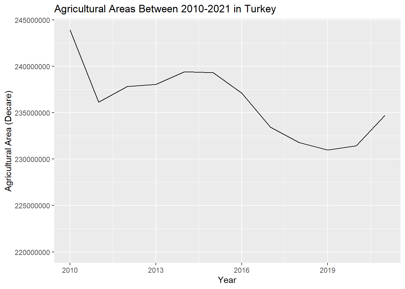
Between 2010-2011, biggest agricultural area lost is happened. In 2011-2015, it seems to be good years for Agriculture in terms of magnitude of the areas. However, after 2015, general trend moves towards to losing the Agricultural areas, after 2019 there seems to be first improvement, interestingly first improvement is in 2020, “the pandemic year” but in general in 11 years, size of the agricultural areas moving downwards.
Yearly agriculture areas
By Province
Add previous decares to the dataframe
df_1 <- tarim %>%
  arrange(province, year) %>%
  group_by(province) %>%
  mutate(prev_decare = lag(decare)) %>%
  ungroup()
head(df_1)
# A tibble: 6 × 5
province province_code year decare prev_decare
<chr> <chr> <dbl> <dbl> <dbl>
1 Adana 1 2010 5506353 NA
2 Adana 1 2011 4962979. 5506353
3 Adana 1 2012 4807968 4962979.
4 Adana 1 2013 4751612. 4807968
5 Adana 1 2014 4982042. 4751612.
6 Adana 1 2015 4887150 4982042.If we look at year by year lost, the biggest lost was in Sivas, 2011 with 2.290.480 decare loss. Second is Kars with 1.628.918, third is Konya with 1.526.849. However, Konya’s total agriculture areas are greater than others. Rate of yearly difference and decare will be another indicator.
df_1 <- df_1 %>%
  mutate(difference = (decare-prev_decare))%>%
  arrange(desc(-1*difference))

head(df_1)
# A tibble: 6 × 6
province province_code year decare prev_decare difference
<chr> <chr> <dbl> <dbl> <dbl> <dbl>
1 Sivas 58 2011 7298275 9588755 -2290480
2 Kars 36 2013 2118640 3747558 -1628918
3 Konya 42 2011 19242360 20769209 -1526849
4 Şanlıurfa 63 2011 11444392. 12591457 -1147065.
5 Yozgat 66 2013 5991422 6985982 -994560
6 Konya 42 2017 18854582 19636340. -781758.If we sort according to rate of difference Ardahan,2014 is the first with 0.44, Kars,2013 with 0.43 and Karabük,2018 with 0.32 are the second and third in terms of yearly agriculture area lost.
df_1 <- df_1 %>%
  mutate(difference_rate = round(difference/prev_decare,2))%>%
  arrange((difference_rate))


head(df_1)
# A tibble: 6 × 7
province province_code year decare prev_decare difference difference_rate
<chr> <chr> <dbl> <dbl> <dbl> <dbl> <dbl>
1 Ardahan 75 2014 329525 588632 -259107 -0.44
2 Kars 36 2013 2118640 3747558 -1628918 -0.43
3 Karabük 78 2018 337488 498499 -161011 -0.32
4 Osmaniye 80 2011 1153635 1664382 -510747 -0.31
5 Sivas 58 2011 7298275 9588755 -2290480 -0.24
6 Kocaeli 41 2018 786927 974696 -187769 -0.19Interestingly, yearly loss is greater in the first half of the decade, but overall loss is increasing year by year, let’s visualise this by adding cumulative loss column.
If we look at total lost, Şanlıurda, Konya ans Sivas are the three big cities
df_p <- df_1 %>%
  group_by(province) %>%
  summarise('TotalDifference'=sum(difference, na.rm=TRUE),'TotalRate'=sum(difference_rate, na.rm=TRUE)) %>%
  arrange(TotalDifference)

knitr::kable(head(df_p),caption = "Total Agriculture Lost Areas by Province 2010-2021")| province | TotalDifference | TotalRate |
|---|---|---|
| Şanlıurfa | -2145906 | -0.15 |
| Konya | -2058950 | -0.10 |
| Sivas | -1771190 | -0.18 |
| Yozgat | -1191803 | -0.16 |
| Kırşehir | -712105 | -0.19 |
| Çorum | -679593 | -0.10 |
df_p <- df_p %>%
  arrange(TotalDifference) %>%
  mutate(TotalDifference=TotalDifference*-1)

ggplot(data=head(df_p,10), aes(x=province, y=TotalDifference)) +
  geom_bar(position="dodge",stat="identity") +
  ggtitle("Total Agriculture Area Loss by Province 2010-2021 - Top 10 Province") +
  theme(text = element_text(size = 10),element_line(size =15),axis.text.x = element_text(angle = 90))+
  xlab("Province") +
ylab("Lost Agricultural Area (Decare)") 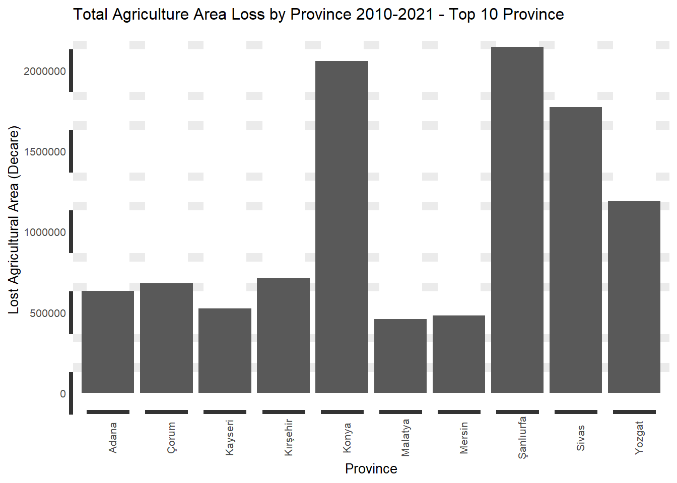
Zonguldak lost 35% of its agricultural areas in 12 years
df_2010 <- df_1 %>%
  filter(year == 2010) %>%
  select(province,year,decare)

df_2021 <- df_1 %>%
  filter(year == 2021) %>%
  select(province,year,decare)

df_join <- inner_join(df_2010,df_2021, by = "province")

df_ttrate <- df_join %>%
  mutate(totaldiffrate = 100*(decare.y-decare.x)/decare.x) %>%
  arrange((totaldiffrate)) %>%
  select (province,totaldiffrate )

knitr::kable(head(df_ttrate),caption = "Total Agricultural Area Loss Rate by Province 2010-2021")| province | totaldiffrate |
|---|---|
| Zonguldak | -34.97663 |
| Batman | -26.32009 |
| Osmaniye | -25.91478 |
| Bartın | -21.38318 |
| Sivas | -18.47153 |
| Yalova | -18.26819 |
ggplot(head(df_ttrate,10), aes(x=province, y=-1*totaldiffrate)) +
  geom_bar(position="dodge",stat="identity") +
  ggtitle("Total Agriculture Area Loss Rate by Province 2010-2021 (Top 10 Province)") +
  theme(axis.text.x = element_text(angle = 90)) +
   ylab("Agricultural Area Loss Rate(%)")+
   xlab("Province")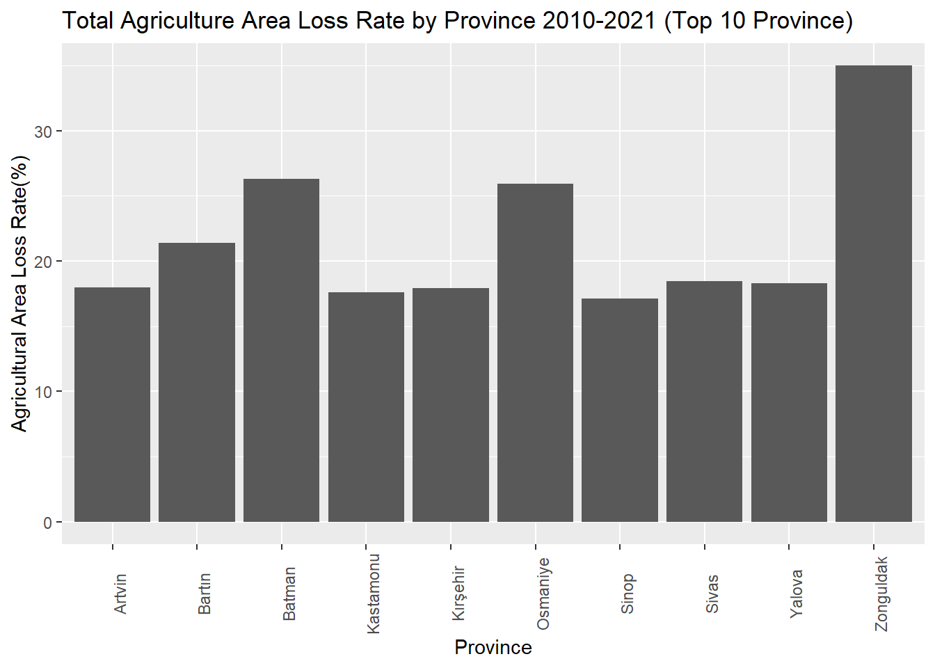
By Region
Adding regions to tarim data
df_r<- merge(x=tarim,y=regions,by="province",all.x = TRUE)
df_region<- df_r%>% select(region,year,decare) %>%
                        group_by(region,year) %>%
                          summarise(Total_Agriarea_in_the_Region=sum(decare))
df_region %>% head()
# A tibble: 6 × 3
# Groups: region [1]
region year Total_Agriarea_in_the_Region
<chr> <dbl> <dbl>
1 Akdeniz Bölgesi 2010 24648042
2 Akdeniz Bölgesi 2011 23881021.
3 Akdeniz Bölgesi 2012 23179936.
4 Akdeniz Bölgesi 2013 23385270.
5 Akdeniz Bölgesi 2014 23545660.
6 Akdeniz Bölgesi 2015 23219406.Add previous decares to the dataframe
df_region_1<- df_region %>%
               arrange(region,year) %>%
                group_by(region) %>%
                 mutate(prev_decare= lag(Total_Agriarea_in_the_Region)) %>%
                   ungroup()
head(df_region_1)
# A tibble: 6 × 4
region year Total_Agriarea_in_the_Region prev_decare
<chr> <dbl> <dbl> <dbl>
1 Akdeniz Bölgesi 2010 24648042 NA
2 Akdeniz Bölgesi 2011 23881021. 24648042
3 Akdeniz Bölgesi 2012 23179936. 23881021.
4 Akdeniz Bölgesi 2013 23385270. 23179936.
5 Akdeniz Bölgesi 2014 23545660. 23385270.
6 Akdeniz Bölgesi 2015 23219406. 23545660.If we look at year by year lost, İç Anadolu had the biggest loses in 2011 and 2017. However İç Anadolu’ total agricultural lands also high as compared to other regions so looking rate of yearly difference would be good indicator to analyze.
df_region_1 <- df_region_1 %>%
       mutate(difference=(Total_Agriarea_in_the_Region-prev_decare)) %>%
         arrange((desc(-1*difference)))
df_region_1
# A tibble: 84 × 5
region year Total_Agriarea_in_the_Region prev_d…¹ diffe…²
<chr> <dbl> <dbl> <dbl> <dbl>
1 İç Anadolu Bölgesi 2011 78302580. 8.14e7 -3.09e6
2 İç Anadolu Bölgesi 2017 77860586. 8.02e7 -2.33e6
3 Güneydoğu Anadolu Bölgesi 2011 30283342. 3.21e7 -1.84e6
4 Doğu Anadolu Bölgesi 2013 24865102. 2.67e7 -1.80e6
5 Marmara Bölgesi 2011 23099178. 2.40e7 -9.03e5
6 Ege Bölgesi 2011 27523248. 2.84e7 -8.74e5
7 Güneydoğu Anadolu Bölgesi 2016 30263398 3.11e7 -8.46e5
8 Akdeniz Bölgesi 2011 23881021. 2.46e7 -7.67e5
9 Akdeniz Bölgesi 2012 23179936. 2.39e7 -7.01e5
10 Güneydoğu Anadolu Bölgesi 2017 29666365 3.03e7 -5.97e5
# … with 74 more rows, and abbreviated variable names ¹prev_decare, ²differenceEastern part of the Turkey loss agricultural land at the highest rate in the first years of decade, “Büyüksehir Yasası” that enacted in the 2012 can be cause of this situation.
df_region_1 <- df_region_1 %>%
          mutate(difference_rate=round(difference/prev_decare,2)) %>%
                   arrange((difference_rate))
head(df_region_1)
# A tibble: 6 × 6
region year Total_Agriarea_in_th…¹ prev_…² diffe…³ diffe…⁴
<chr> <dbl> <dbl> <dbl> <dbl> <dbl>
1 Doğu Anadolu Bölgesi 2013 24865102. 2.67e7 -1.80e6 -0.07
2 Güneydoğu Anadolu Bölgesi 2011 30283342. 3.21e7 -1.84e6 -0.06
3 İç Anadolu Bölgesi 2011 78302580. 8.14e7 -3.09e6 -0.04
4 Marmara Bölgesi 2011 23099178. 2.40e7 -9.03e5 -0.04
5 İç Anadolu Bölgesi 2017 77860586. 8.02e7 -2.33e6 -0.03
6 Ege Bölgesi 2011 27523248. 2.84e7 -8.74e5 -0.03
# … with abbreviated variable names ¹Total_Agriarea_in_the_Region,
# ²prev_decare, ³difference, ⁴difference_rateLet’s look at the overall lose between 2010-2021 by region.In this case some regions interestingly increase their agricultural lands
df_region_overall <- df_region_1 %>%
                      group_by(region) %>%
                         summarise("Total_Difference"=sum(difference,na.rm=TRUE),"Total_Rate"=sum(difference_rate,na.rm = TRUE)) %>%                             arrange(Total_Rate)
knitr::kable(df_region_overall,caption = "Total Agriculre Lost Areas by Region 2010-2021")| region | Total_Difference | Total_Rate |
|---|---|---|
| Güneydoğu Anadolu Bölgesi | -3003875.0 | -0.11 |
| Akdeniz Bölgesi | -2254601.0 | -0.09 |
| İç Anadolu Bölgesi | -4191358.8 | -0.05 |
| Ege Bölgesi | -432585.9 | -0.02 |
| Karadeniz Bölgesi | -557447.5 | -0.01 |
| Marmara Bölgesi | 104406.2 | 0.01 |
| Doğu Anadolu Bölgesi | 1122184.3 | 0.04 |
Visualization…
ggplot(data=df_region_overall,aes(x=region,y=Total_Difference,fill=region))+
  geom_bar(position = "dodge",stat="identity")+
  ggtitle("Total Agriculture Area Loss by Region 2010-2021")+
  theme(text = element_text(size=10),element_line(size=15),axis.text.x=element_text(angle=90))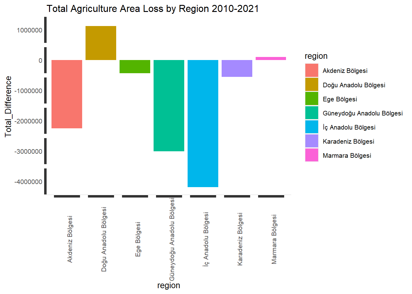
Distribution of Agricultural Production
Fruits
meyve_dekar <-
  meyve %>%
  filter(year==2021 & unit=='Dekar'  & main_type=='Toplu Meyveliklerin Alanı')


total = sum(meyve_dekar[, 'production'],na.rm=TRUE)

grouped_data <- meyve_dekar %>%
  group_by(product_name) %>%
  summarise(TotalbyName = sum(production,na.rm=TRUE)) %>%
  mutate(rate = round((TotalbyName/total)*100,4))

plot_data <- grouped_data %>%
  mutate(rank = rank(-TotalbyName),
         product_name = ifelse(rank <= 10, product_name, 'Other'))
p <- plot_ly(plot_data, labels = ~product_name, values = ~TotalbyName, type = 'pie',textposition = 'outside',textinfo = 'label+percent') %>%
layout(title = 'Top 10 Fruit Products (in Decare) in Turkey in 2021',
xaxis = list(showgrid = FALSE, zeroline = FALSE, showticklabels = FALSE),
yaxis = list(showgrid = FALSE, zeroline = FALSE, showticklabels = FALSE))
pVegetables
sebze_df <- sebze %>%
  filter(year==2021 & unit=='Dekar'  & main_type=='Ekilen Alan')

total = sum(sebze_df [, 'decare'],na.rm=TRUE)

grouped_data <- sebze_df %>%
  group_by(product_name) %>%
  summarise(TotalbyName = sum(decare,na.rm=TRUE)) %>%
  mutate(rate = round((TotalbyName/total)*100),4)

plot_data_v <- grouped_data %>%
  mutate(rank = rank(-TotalbyName),
         product_name = ifelse(rank <= 10, product_name, 'Other'))
p <- plot_ly(plot_data_v, labels = ~product_name, values = ~TotalbyName, type = 'pie',textposition = 'outside',textinfo = 'label+percent') %>%
layout(title = 'Top 10 Vegetable Products (in Decare) in Turkey in 2021',
xaxis = list(showgrid = FALSE, zeroline = FALSE, showticklabels = FALSE),
yaxis = list(showgrid = FALSE, zeroline = FALSE, showticklabels = FALSE))
pGrain
tahil_df <-  tahil %>%
  filter(year==2021 & unit=='Dekar' & main_type=='Ekilen Alan')

total = sum(tahil_df[, 'decare'],na.rm=TRUE)

grouped_data <- tahil_df %>%
  group_by(product_name) %>%
  summarise(TotalbyName = sum(decare,na.rm=TRUE)) %>%
  mutate(rate = round((TotalbyName/total)*100),2)

plot_data_g <- grouped_data %>%
  mutate(rank = rank(-TotalbyName),
         product_name = ifelse(rank <= 10, product_name, 'Other'))
p <- plot_ly(plot_data_g, labels = ~product_name, values = ~TotalbyName, type = 'pie',textposition = 'outside',textinfo = 'label+percent') %>%
layout(title = 'Top 10 Grain Products(as Decare) in Turkey in 2021',
xaxis = list(showgrid = FALSE, zeroline = FALSE, showticklabels = FALSE),
yaxis = list(showgrid = FALSE, zeroline = FALSE, showticklabels = FALSE))
pYearly Grain/Fruit/Vegetable Production Areas
Grain production areas were decreasing until 2019, after 2019, it is increasing slightly like agricultural areas
df_gra <- tahil %>%
  filter(unit=='Dekar' & main_type=='Ekilen Alan') %>%
  group_by(year)%>%
  summarize(total_gra_decare = sum(decare, na.rm = TRUE))

ggplot(data=df_gra, aes(x=year, y=total_gra_decare)) +
  geom_line() +
  geom_smooth(method = "lm", formula = y ~ poly(x, 3), se = FALSE) +
  labs(x ="Year",y="Decare") +
  ggtitle("Total Grain Agriculture Areas(Decare) Between 2010-2021")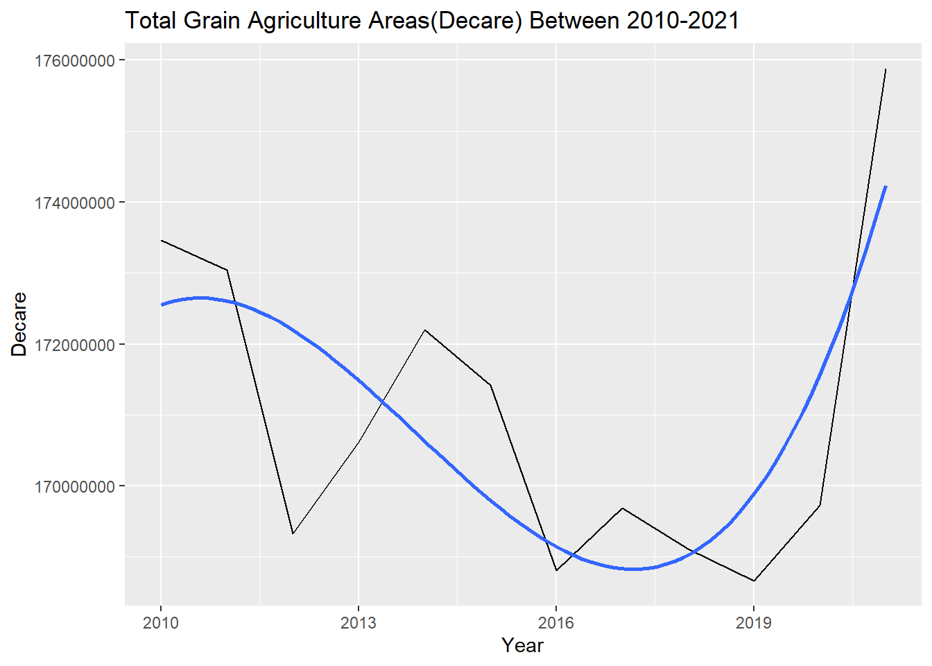
Fruit production areas are increasing slightly unlike agricultural areas
df_meyve <- meyve %>%
  filter(unit=='Dekar' & main_type=='Toplu Meyveliklerin Alanı') %>%
  group_by(year)%>%
  summarize(total_gra_decare = sum(production, na.rm = TRUE))

ggplot(data=df_meyve, aes(x=year, y=total_gra_decare)) +
  geom_line() +
  geom_smooth(method = "lm", formula = y ~ poly(x, 3), se = FALSE) +
  labs(x ="Year",y="Decare") +
  ggtitle("Total Fruit Agriculture Areas(Decare) Between 2010-2021")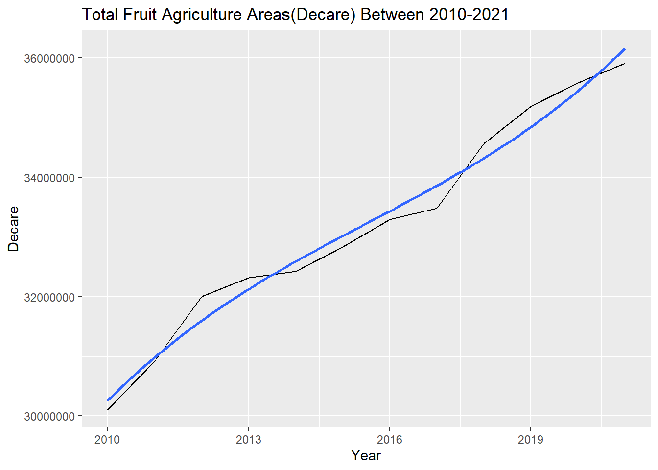
meyve_sort <- meyve %>% arrange(year)

meyve_analiz <- meyve_sort %>%
  filter(unit=='Dekar'  & main_type=='Toplu Meyveliklerin Alanı') %>%
  group_by(year,product_name)%>%
  summarize(total_decare = sum(production, na.rm = TRUE)) %>%
  arrange(product_name,year) %>%
  ungroup()


meyve_sort_analiz <- meyve_analiz %>%
  mutate(prev_dekar=lag(total_decare))  %>%
  mutate(difference_with_prev_year =total_decare-prev_dekar ) %>%
  filter(year>2010) %>%
  arrange(desc(difference_with_prev_year))

knitr::kable(head(meyve_sort_analiz),caption = "The Top Fruits in Terms of Yearly Increased Agricultural Areas ")| year | product_name | total_decare | prev_dekar | difference_with_prev_year |
|---|---|---|---|---|
| 2012 | Şam Fıstığı Antep Fıstığı | 2835517 | 2338368 | 497149 |
| 2018 | Yağlık Zeytinler Zeytinyağı Üretimi İçin | 6544561 | 6195707 | 348854 |
| 2011 | Fındık | 6969643 | 6678649 | 290994 |
| 2018 | Şam Fıstığı Antep Fıstığı | 3545003 | 3288041 | 256962 |
| 2019 | Sofralık Zeytinler | 2341306 | 2099722 | 241584 |
| 2016 | Şam Fıstığı Antep Fıstığı | 3134316 | 2914179 | 220137 |
df_sebze <- sebze %>%
  filter(unit=='Dekar' & main_type=='Ekilen Alan') %>%
  group_by(year)%>%
  summarize(total_gra_decare = sum(decare, na.rm = TRUE))


ggplot(data=df_sebze, aes(x=year, y=total_gra_decare)) +
  geom_line() +
  geom_smooth(method = "lm", formula = y ~ poly(x, 3), se = FALSE) +
  labs(x ="Year",y="Decare") +
  ggtitle("Total Vegetable Agriculture Areas(Decare) Between 2010-2021")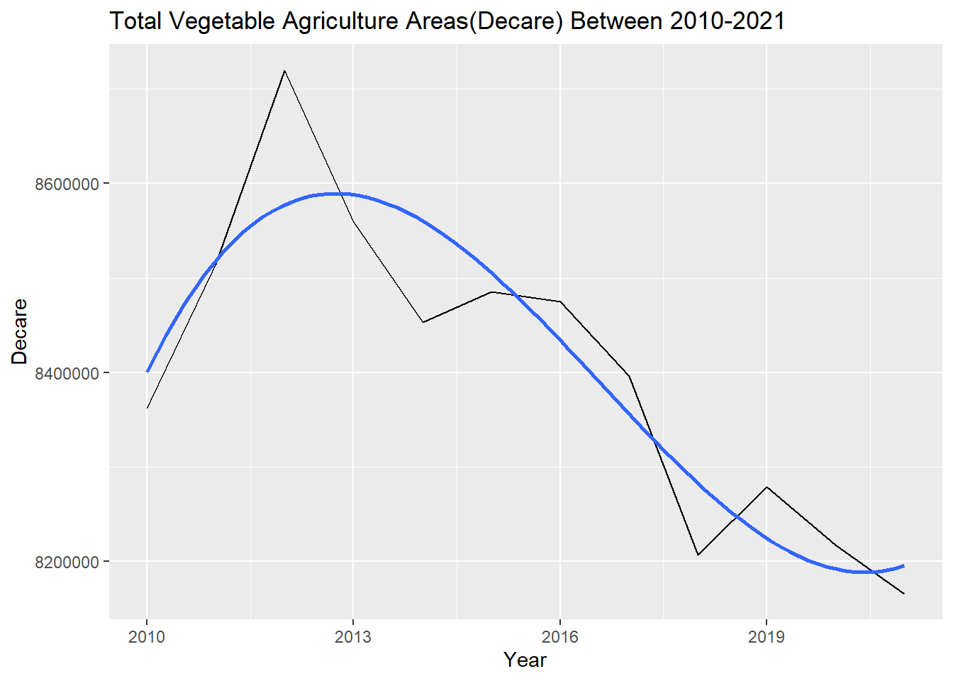
Above analysis show that, increase in the agricultural areas after 2019 due to fruit (mostly nuts) and grain production
Climate Indicators and Agriculture Areas
In this section we will compare the yearly average temperatures with the agriculture areas. Weather data is gathered from TradingEconomics.
temperature = read_excel("data//temp.xlsx")


df <- tarim %>%
  group_by(year) %>%
  summarise(TotalDecareNormalized=sum(decare)/ 20000000)


df_t <- df %>%
  inner_join(temperature,by = "year")

ggplot(df_t, aes(year)) +
  geom_line(aes(y = TotalDecareNormalized, colour = "Total Agricultural Area in Decare (1/20000000)")) +
  geom_line(aes(y = temperature, colour = "Temperature")) +
  ylab(NULL) +
ggtitle("Average Temperature vs Total Agricultural Area") 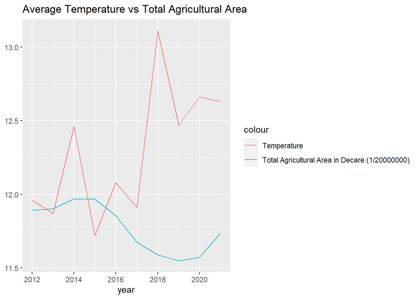
Increase in average temperature in Turkey in 2018, also coincides with the decrease in Agricultural area. Note that we need further statistical tests to show the relation between, this presentations only shows the raw data. However, *there are evidences suggesting that rising temperatures due to climate change can have negative impacts on agriculture, including crop yields and the productivity of livestock.
CO2 emission is also an important metric for measuring the climate change. CO2 emissions (metric tons per capita) Carbon dioxide emissions are those stemming from the burning of fossil fuels and the manufacture of cement. They include carbon dioxide produced during consumption of solid, liquid, and gas fuels and gas flaring.
WorldBank launches the CO2 emissions (metric tons per capita) data for every country. I used WorldBank
Note that, Data consists of the CO2 emission for 2009-2019
co2 = read_excel("data//co2.xlsx")


df_t$year<-as.character.Date(df_t$year)
df_t_c <- df_t %>%
  inner_join(co2, by='year')

ggplot(df_t_c, aes(year)) +
  geom_line(aes(y = TotalDecareNormalized, colour = "Total Decare (1/20000000)", group=1)) +
  geom_line(aes(y = CO2emissions, colour = "CO2 Emission(Ton Per Capita)", group=2)) +
  geom_line(aes(y = temperature, colour = "Temperature", group=3)) +
  ylab(NULL) +
ggtitle("Average Temperature, CO2 Emission and Total Agricultural Area in Turkey") 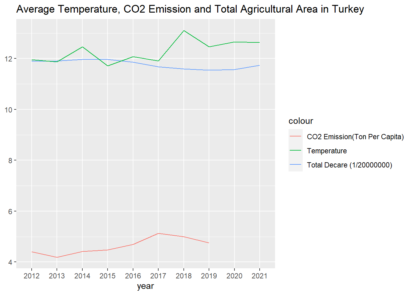
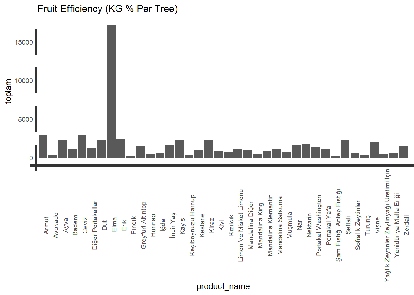
Most efficient Fruits in Turkey
Production in kg per tree is as follows, is seems Apple is the winner here too.
df_e <- meyve %>%
  filter(str_trim(unit)=='Kg/Meyve Veren Ağaç')%>%
  group_by(product_name,unit) %>%
  summarise(toplam = sum(production, na.rm = TRUE)) %>%
  arrange(desc(toplam))

knitr::kable(head(df_e),caption = "Fruit Efficiency (KG % Per Tree)")| product_name | unit | toplam |
|---|---|---|
| Elma Starking | Kg/Meyve Veren Ağaç | 41119 |
| Elma Golden | Kg/Meyve Veren Ağaç | 40949 |
| Diğer Elmalar | Kg/Meyve Veren Ağaç | 33089 |
| Armut | Kg/Meyve Veren Ağaç | 31858 |
| Elma Granny Smith | Kg/Meyve Veren Ağaç | 30369 |
| Elma Amasya | Kg/Meyve Veren Ağaç | 30143 |
Let’s group all fruits containing “Elma” under the Elma.
meyve_group <- meyve

meyve_group$product_name <- gsub(".*Elma.*", "Elma", meyve$product_name)


df_elma <- meyve_group %>%
  filter(str_trim(unit)=='Kg/Meyve Veren Ağaç')%>%
  group_by(year,product_name,unit) %>%
  summarise(toplam = sum(production, na.rm = TRUE)) %>%
  arrange(year,desc(toplam))
df_elma
# A tibble: 453 × 4
# Groups: year, product_name [453]
year product_name unit toplam
<dbl> <chr> <chr> <dbl>
1 2010 "Elma" Kg/Meyve Veren Ağaç 16454
2 2010 "Ceviz " Kg/Meyve Veren Ağaç 2794
3 2010 "Armut " Kg/Meyve Veren Ağaç 2532
4 2010 "Ayva " Kg/Meyve Veren Ağaç 2176
5 2010 "Erik " Kg/Meyve Veren Ağaç 2167
6 2010 "Kiraz " Kg/Meyve Veren Ağaç 2126
7 2010 "Şeftali " Kg/Meyve Veren Ağaç 2040
8 2010 "Dut " Kg/Meyve Veren Ağaç 2005
9 2010 "Kayısı " Kg/Meyve Veren Ağaç 1940
10 2010 "Vişne " Kg/Meyve Veren Ağaç 1802
# … with 443 more rowsggplot(data=df_elma, aes(x=product_name, y=toplam)) +
geom_bar(position="dodge",stat="identity") +
ggtitle("Fruit Efficiency (KG % Per Tree)") +
theme(text = element_text(size = 10),element_line(size =15),axis.text.x = element_text(angle = 90))