Show the code
library(tidyverse)
library(dplyr)
library(readxl)
library(lubridate)
library(tidyr)
library(zoo)
library(janitor)
library(reactable)
library(data.table)
library(ggplot2)library(tidyverse)
library(dplyr)
library(readxl)
library(lubridate)
library(tidyr)
library(zoo)
library(janitor)
library(reactable)
library(data.table)
library(ggplot2)We are importing construction cost index, Turnover rate, usd to tl exchange rate, House sales to foreigners, House Sales by Province data sets.
ConsIndex <- readRDS("Datards/ConsIndex.rds")
Turnover <- readRDS("Datards/Turnover.rds")
House_sales_to_foreigners_month <- readRDS("Datards/House_sales_to_foreigners_month.rds")
House_sales_to_foreigners_year <- readRDS("Datards/House_sales_to_foreigners_year.rds")

monthly_usd_to_try <- read_excel("data/monthly_usd_to_try.xls")
monthly_usd_to_try$month <- as.Date(monthly_usd_to_try$month)
monthly_usd_to_try$month <- format(monthly_usd_to_try$month,"%Y-%b-%d")

PATH <- "data/House Sales by Provinces.xls"
house_sales_by_provinces <- read_excel(PATH, range = cell_rows(14:129), col_names = names(read_excel(PATH, skip = 2)))

total_sales_by_year <- aggregate(house_sales_by_provinces[3], house_sales_by_provinces[1], FUN=sum)

House_sales_to_foreigners_month <- read_excel("data/House sales to foreigners.xls",
                                                   sheet = "Month")
House_sales_to_foreigners_month$Month <- match(House_sales_to_foreigners_month$Month, month.name)

House_sales_to_foreigners_month$Date <- as.yearmon(paste(House_sales_to_foreigners_month$Year, House_sales_to_foreigners_month$Month), "%Y %m")ggplot(House_sales_to_foreigners_month, aes(Date)) +
geom_line(aes(y = Total, colour = "Total")) +
geom_line(aes(y = `Sales to foreigners`, colour = "Sales To Foreigners"))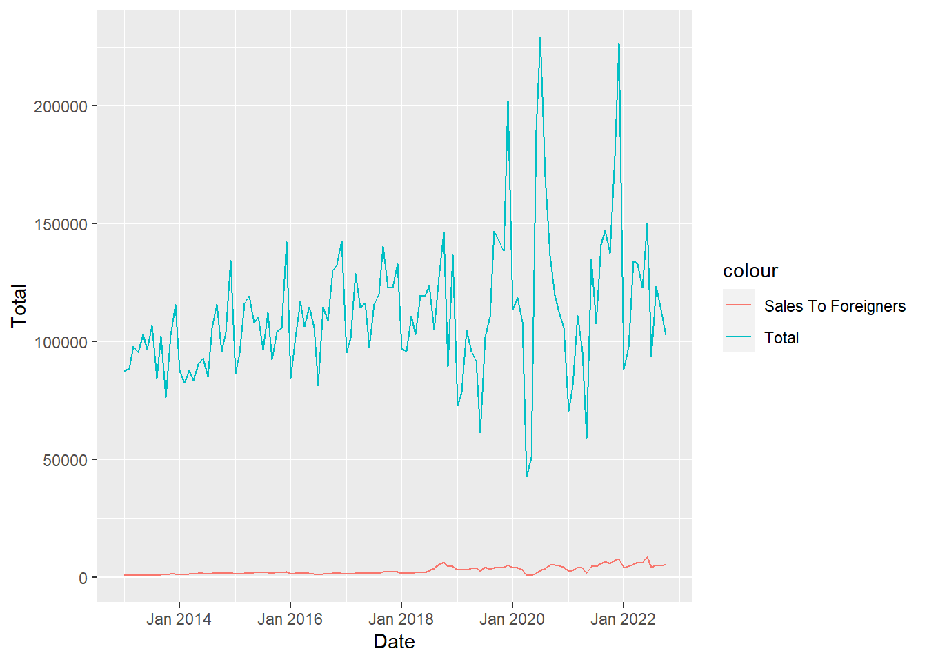
ggplot(House_sales_to_foreigners_month, aes(Date)) +
  geom_line(aes(y = `Share (%)`, colour = "Share (%)"))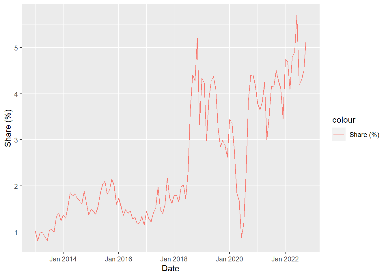
Finding construction cost index yearly mean to compare
ConsIndexYear <- ConsIndex %>% group_by(Year) %>% summarise(Construction_cost_mean = mean(index, na.rm = TRUE))
TurnoverYear <- Turnover %>% group_by(Year) %>% summarise(Turnover_mean = mean(`seasonal and calendar adjusted
Index`))

ConsIndexYear %>% left_join(TurnoverYear, by = "Year") %>% ggplot(aes(Year)) +
  geom_line(aes(y = Construction_cost_mean, colour = "Construction cost mean")) +
  geom_line(aes(y = Turnover_mean, colour = "Turnover mean"))+
  labs(title="Construction cost and Turnover index yearly mean comparison")+
  xlab("Year") +
  ylab("Index")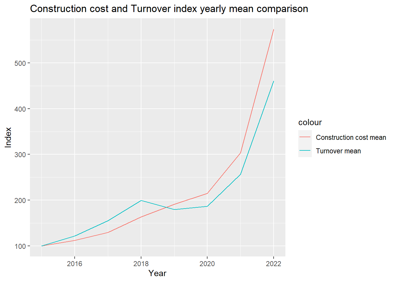
house_sales_by_provinces  <- house_sales_by_provinces  %>%
    fill(colnames(house_sales_by_provinces[1]), .direction = "downup")

# Creating Time Series Object for House Sales by Proviences
total_hs_ts <- ts(house_sales_by_provinces[3],start=c(2013,1),frequency=12)

options(repr.plot.width=21, repr.plot.height=8)
plot(total_hs_ts)monthly_usd_to_try <- read_excel("data/monthly_usd_to_try.xls")
monthly_usd_to_try$month <- as.Date(monthly_usd_to_try$month)
colnames(monthly_usd_to_try) <- c("date","value")
ggplot(data=monthly_usd_to_try, aes(x=date, y=value, group=1)) +
geom_line()+
geom_point()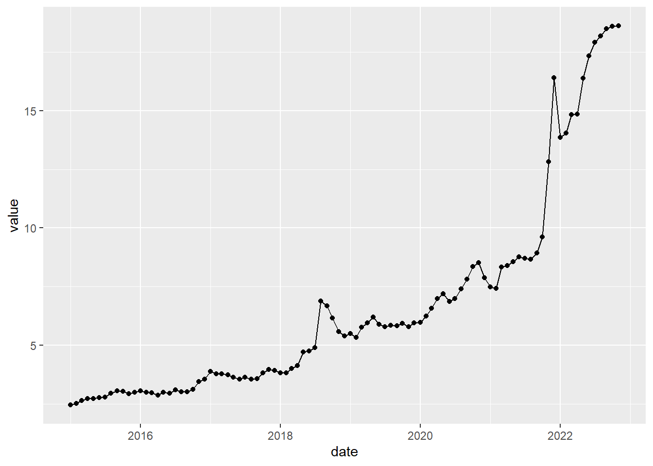
construction_cost_index <- read_excel("data/construction_cost_index_by_industries_and_cost_groups_preprocessed.xls")


construction_cost_index$date <- as.Date(construction_cost_index$date)
colnames(construction_cost_index) <- c("date","cost_type","value","material","labour")

cost_index = construction_cost_index %>%
  filter(cost_type=="construction") %>%
  group_by(date) %>%
  summarize(value=sum(value))

ggplot(data=cost_index, aes(x=date, y=value, group=1)) +
  geom_line()+
  geom_point()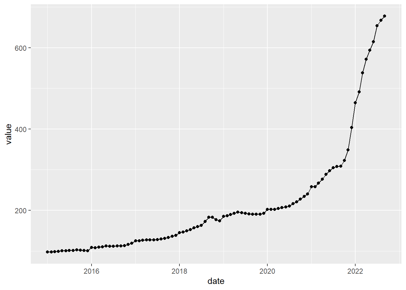
After 2017, Iran overtakes Iraq. There is a high increase in Russia as we move from 2021 to 2022. We assume the reason is Ukraine - Russian war.
HSTFBN <- read_excel("data/HSTFBN.xls", sheet = "FOREIGNERS BY NATIONALITIES")

total_sale_by_country <- HSTFBN %>% group_by(year,country) %>% filter(country %in% c("Russia","Iran", "Iraq")) %>% summarise(sum=sum(total))
`summarise()` has grouped output by 'year'. You can override using the
`.groups` argument.ggplot(data=total_sale_by_country,aes(x=year,y=sum,fill=country)) +
geom_bar(stat="identity",position = "dodge")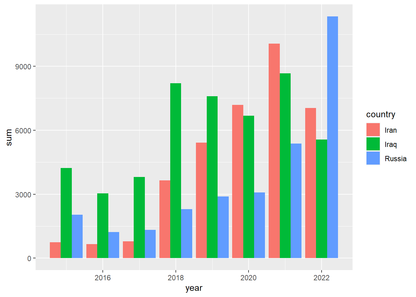
house_sales_by_districts_preprocessed <- read_excel("data/house_sales_by_districts_preprocessed.xls")

house_sales <- house_sales_by_districts_preprocessed %>%
  group_by(year) %>%
  summarise(morgaged=sum(mortgaged), total=sum(total), first_hand=sum(first_hand), second_hand=sum(second_hand))


ggplot(data=house_sales,aes(x=year),group = 1 ) +
  geom_line(aes(y=morgaged,color='morgaged')) +
  geom_line(aes(y=total,color='total'))+
  xlab("Year")+
  ylab("Values")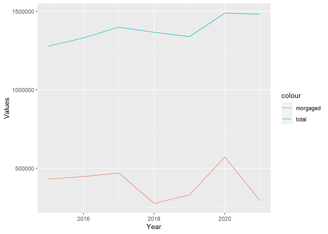
house_sales_by_districts_preprocessed <- read_excel("data/house_sales_by_districts_preprocessed.xls")

house_sales <- house_sales_by_districts_preprocessed %>%
  group_by(year) %>%
  summarise(morgaged=sum(mortgaged), total=sum(total), first_hand=sum(first_hand), second_hand=sum(second_hand))


ggplot(data=house_sales,aes(x=year),group = 1 ) +
  geom_line(aes(y=first_hand,color='first_hand')) +
  geom_line(aes(y=second_hand,color='second_hand')) +
  xlab("Year")+
  ylab("Values")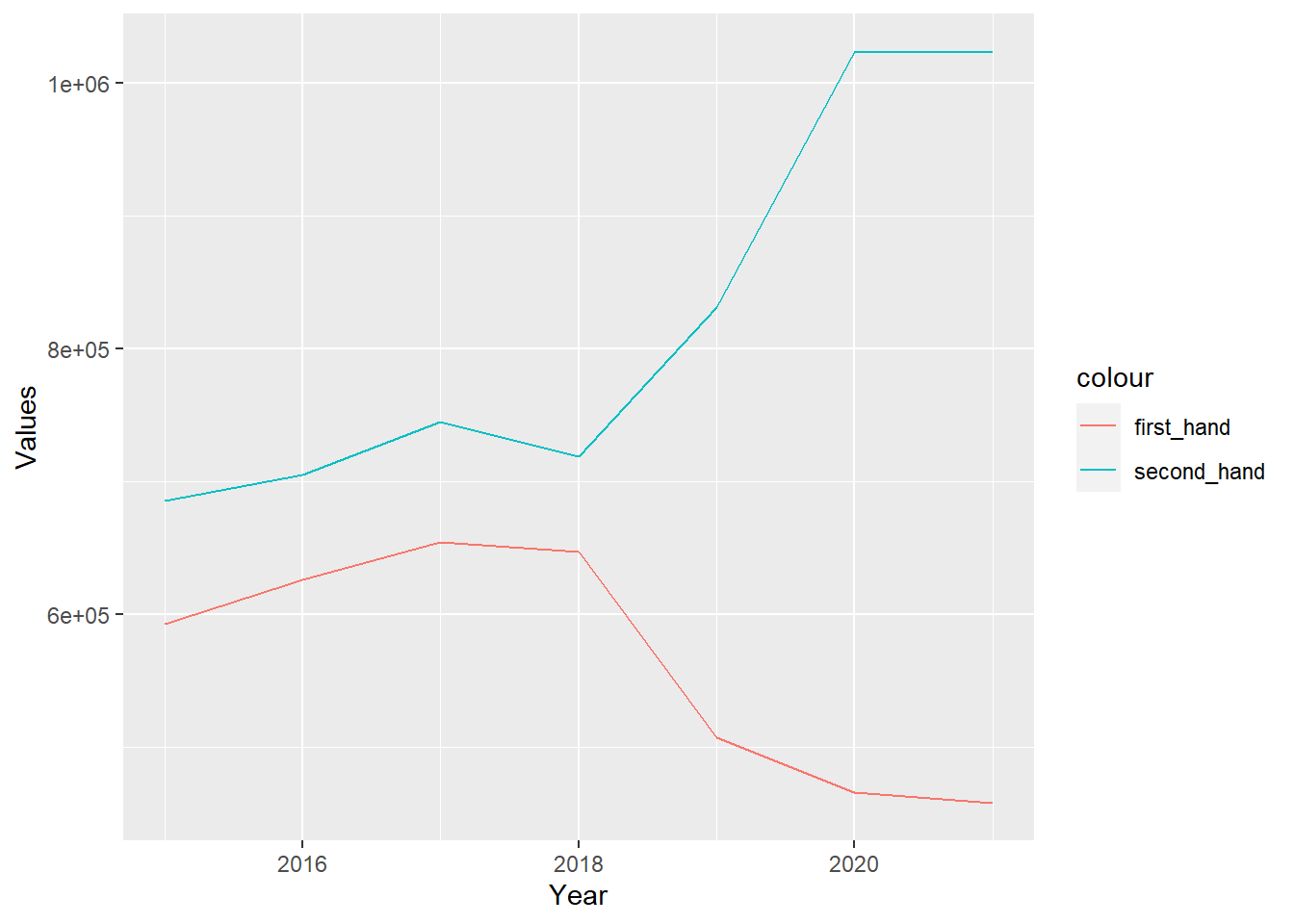
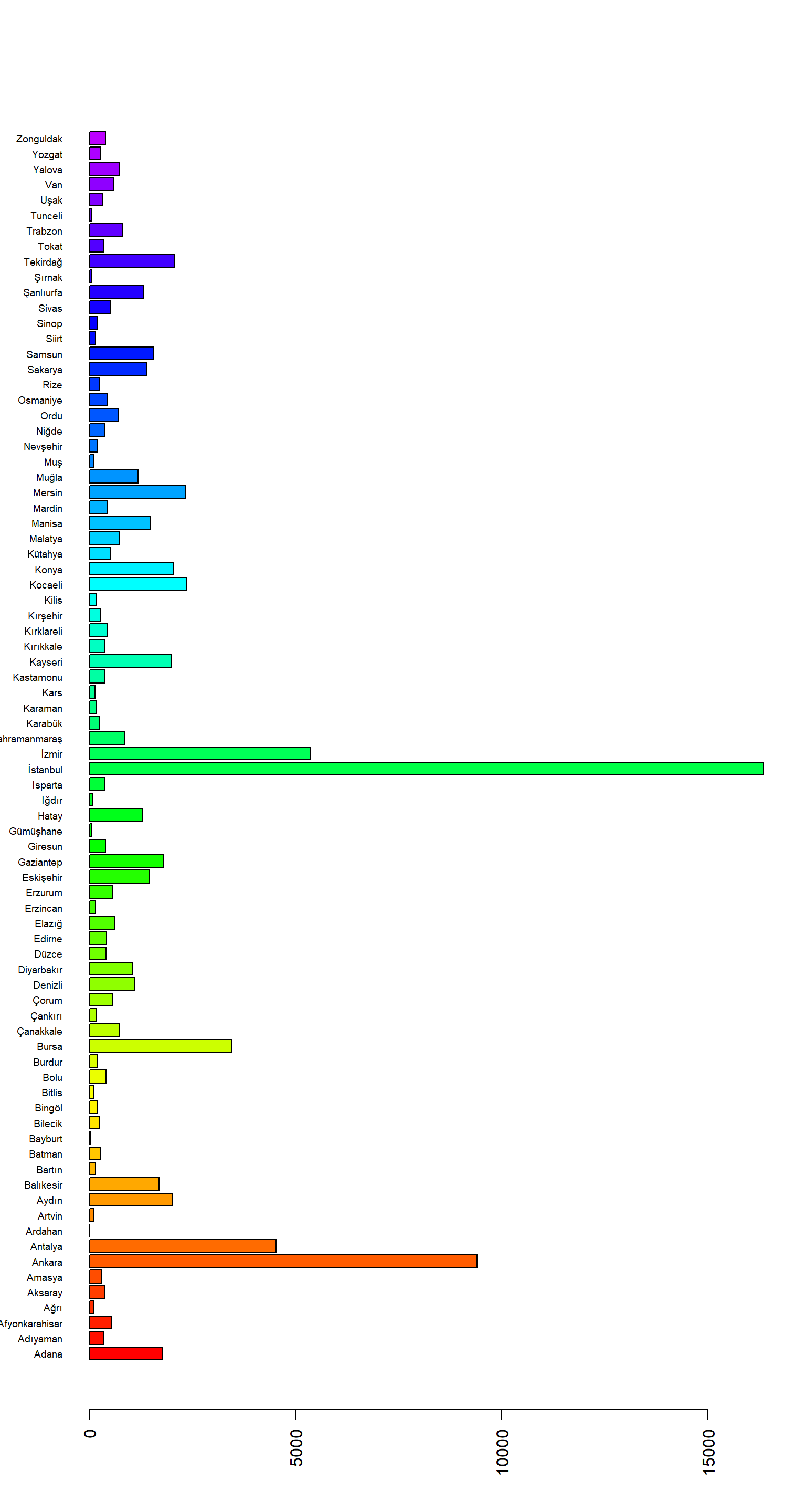
annual_avg_hs <- slice(house_sales_by_provinces %>%
    group_by(house_sales_by_provinces[1]) %>%
    summarize_if(is.numeric,sum,na.rm = TRUE), 1:(n()-1))[3:82] %>%
    summarize_if(is.numeric,mean,na.rm = TRUE)


barplot(unlist(annual_avg_hs), col = rainbow(100), las=2, cex.names=.6, horiz = TRUE)