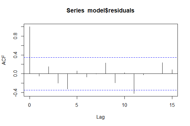
library(stats)
model <- lm(mpg~drat, data=mtcars)
acf(model$residuals, type="correlation")1 BDA-503 Data Analytics Essentials: Assignment 1
1.1 Introducing Myself
Hi. This is Yigit. I was born in Ankara, in 1990. I obtained my undergraduate degree from Department of Economics at Bogazici University. After my graduation, I passed the three-stage examination process of Turkiye İş Bankası and started as assistant auditor, which gave me a solid background in banking sector such as the business structure of both headquarters, branches, and their subsidiaries, risk analysis of loan portfolios of corporates and SMEs.
As an advancement in my career, I passed the researcher examination of The Central Bank of Republic of Turkey (CBRT) Turkey, and started to work as a researcher. Currently, I am working in Markets Department as an assistant economist in CBRT. My fields of interests consist of macroeconomics, financial modelling and empirical asset pricing in general. To be more specific, most of my studies are about pricing of financial derivatives. Some of my papers with my colleagues are The Determinants of Currency Risk Premium in Emerging Market Countries, A Measure of Turkey’s Sovereign and Banking Sector Credit Risk: Asset Swap Spreads.
As we live in a world of massive data, being able to use them efficiently is crucial. The processes of collecting data, analysing them, illustrating the results and preparing automated reports as well as being able to apply modern machine learning techniques to macro-financial data are the main accomplishments I want to make at the end of the Big Data Analytics program.
You can reach me via my linkedin page.
1.2 UseR-2022 Videos
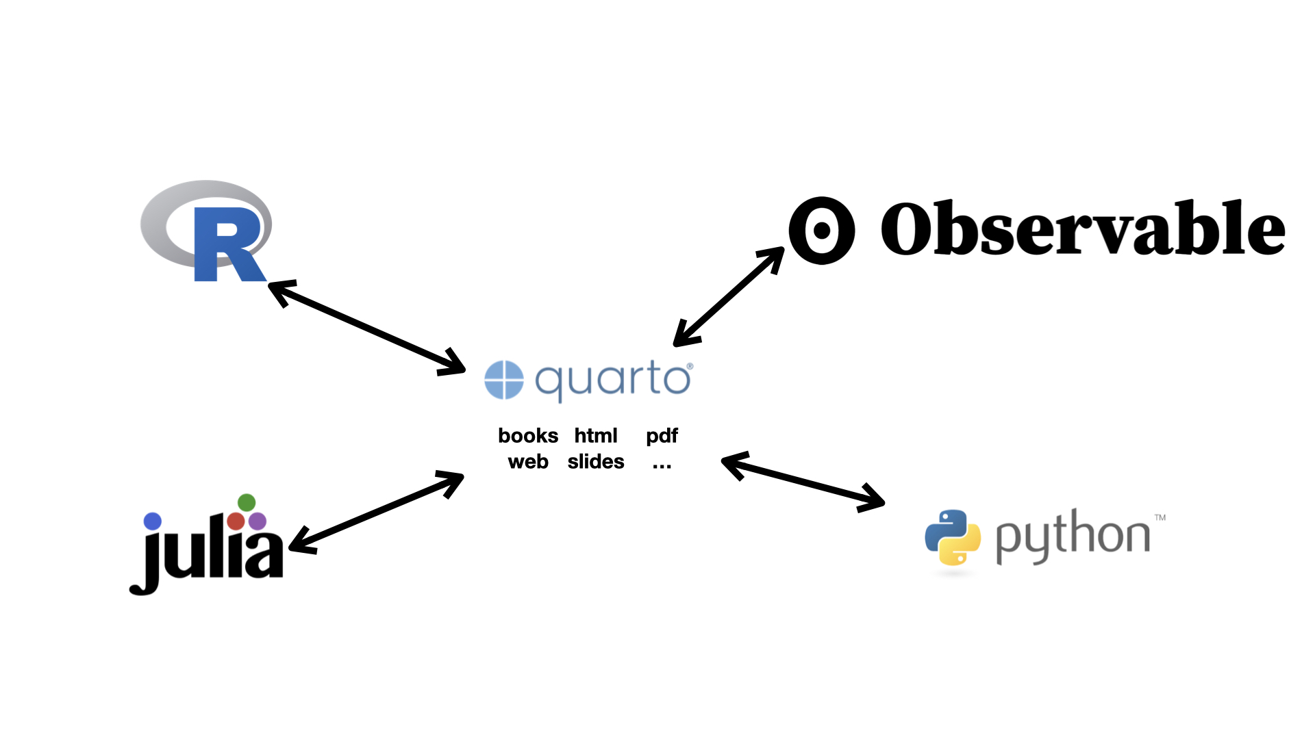
This section summarise the speech given by Devin Pastoor titled Websites & Books & Blogs, oh my! Creating Rich Content with Quarto during RStudio Global 2022 conference. I chose this topic as Quarto is the main tool for scripting our coursework in our course this semester and “Devin Pastorr” decribes the novalties Quarto brings to business and academics.
The opportunity to build on a unit of Rmarkdown into more complex content such as websites, books and blogs required additional programs to which lots of effort had been made.In this regard, many different packages/programs had been introduced, such as bookdown or blogdown, which results in the seperation of the comnnutiy.
Devin Pastoor emphasizes the signficance of Quarto as it
- unifies teams across language boundaries and procedural differences and
- gives unparalelled ability to processing and producing the content in various forms.
1.3 Miscallaneous R-Posts
In this section, 3 R-posts are chosen to be outlined.
1.3.1 Difference between R and Python
This post discusses the main properties of R and Python and overview their similarities and differences.

R
- R has undergone two decades of development by statisticians and academics.
- It is the preferred choice for statistical analysis, especially for specialist analytical work, thanks to its extensive library.
Python
- Python is a tool for large-scale machine learning deployment and implementation.
- It is able to perform many of the same activities as R, including data manipulation, engineering, feature selection, web scraping, and app development.
Comparing R & Python;
Their similarities include - Both the open-source programming languages R and Python have a sizable user base - Their individual catalogs are always being updated with new libraries or tools. - Both can manage very large databases.
They differ in certain ways such that: - Python offers a more all-encompassing approach to data science whereas R is primarily employed for statistical analysis. - Python users tend to be programmers and developers, whereas R users are primarily academics and R&D experts. - R is initially challenging to learn, but Python is linear and simple to understand.
1.3.2 Visualizing OLS Linear Regression Assumptions in R
This post illustrates some of the assumptions of classical linear regression model which are:
- Weak Exogeneity
- Linearity
- Constant Variance
- Independence of Errors
- Lack of Perfect Multicollinearity
Linearity
Linearity is likely the easiest assumption to visualize as you can simply use the following code snippet to quickly create a scatterplot.

Multicollinearity
The convenient way to search for existence of correlation between variables it to plot correlation matrix.

Autocorrelation
Creating autocorrelation function plot via stats library in R helps detect existence of autocorrelation among error terms statistically.
1.3.3 The K-Means Clustering Algorithm Intuition Demonstrated In R
This section presents a blogpost by Vincent Tabora demonstrating the K-Means Clustering Algorithm, which is an unsupervised learning method that aims to identify clusters or groups within a given dataset. Each cluster will have a centroid containing the data points or vectors closest to it. It is an iterative process that does not have a predetermined value of how many times to perform.
Simplified steps for K-Means Clustering are:
1- Choose the number of clusters K.
2- Select random K points or the centroids.
3- Assign the data points to their closest centroids by Euclidean distance.
4- Reassign data points if they fall closer to another cluster. Compute and place new centroids in the cluster.
5- Repeat step 3 and 4 until all data points can be grouped in a cluster without re-assigning.
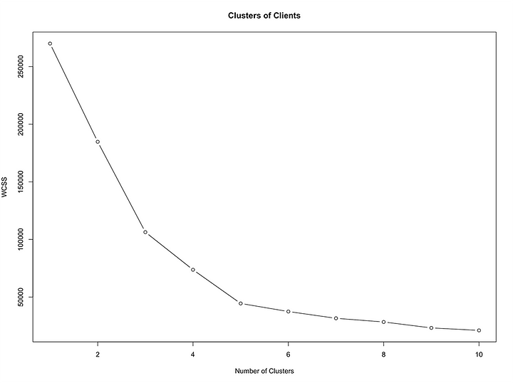
Optimal Number of Clusters
A technique called the Elbow Method to find the optimal number of clusters in dataset.
wcss <- vector()
for (i in 1:10) wcss[i] <- sum(kmeans(X, i)$withinss)
plot(1:10, wcss, type = 'b', main = paste('Clusters of Clients'), xlab = 'Number of Clusters', ylab = 'WCSS')
The rule is to choose the point at which the plot starts decreasing in a linear fashion.
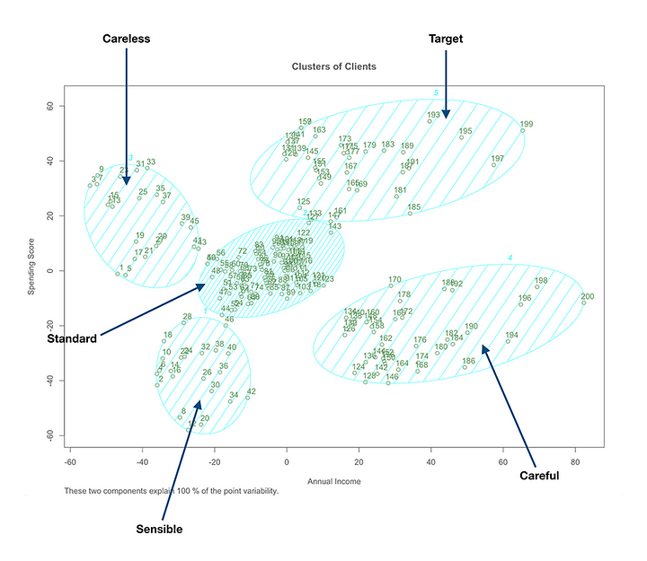
Clustering Algorithm
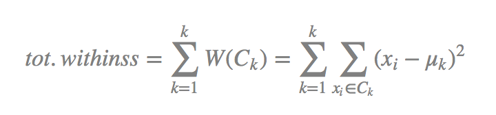
Dataset is into groups using K-Means Clustering. The formula used in K-Means uses the within-cluster sum of squares (wcss) for measuring the compactness of the cluster.
Each of the observations (Xi) are assigned to a cluster such that the sum of squares (SS) distance of the observations to their assigned cluster centers (μk) are at a minimum.
kmeans <- kmeans(X, 5, iter.max = 300, nstart = 10)
library(cluster)
clusplot(X,
         kmeans$cluster,
         lines = 0,
         shade = TRUE,
         labels = 2,
         plotchar = FALSE,
         span = TRUE,
         main = paste('Clusters of Clients'),
         xlab = 'Annual Income',
         ylab = 'Spending Score')
The result will be to gather insights on the dataset in order to make informed decisions.
What the data shows is that people with high incomes will not always spend higher than everyone else, and there are people with low income who are big spenders.