RoadRunneR Term Project

1-Key Takeaways

We have contacted with TUIK-Turkish Statistical Institute- for obtaining a better formatted data set than the ones on their internet site
What our aim is to inspect the housing sales data for at least the last 3 years with price, mortgage credits information, demographical information about the buyer and the province information as the city
We analyzed the numbers of house sales to foreigners and distributions to the major cities in Turkey
We also analyzed the numbers of house sales by gender and inspect which cities have more female owner by ratio than others.

2-Data Extraction and Cleaning

Required libraries for analysis are loaded below

knitr::opts_chunk$set(echo = TRUE)
library(tidyverse)
library(sp)
library(ggplot2)
library(readr)
library(tibble)
library(tidyr)
library(purrr)
library(rvest)
library(xml2)
library(reshape2)
library(mapproj)
library(wordcloud)
library(tm)
library(ggthemes)
library(scales) # Needed for formatting y-axis labels to non-scientific type
library(sqldf)

Data tables published to GitHub, url assigned, and files read below

file_url<- paste('https://github.com/pjournal/mef03g-road-runner/blob/master/TUIK-DATA/House_Sales_Foreigners.csv?raw=true', sep='')

file_url_gender<- paste('https://github.com/pjournal/mef03g-road-runner/blob/master/TUIK-DATA/House_Sales_Gender.csv?raw=true', sep='')

file_url_province<- paste('https://raw.githubusercontent.com/pjournal/mef03g-road-runner/master/TUIK-DATA/House_Sales_Provinced_Based.csv?raw=true', sep='')


# Reading foreigners data from the url
raw_data <- read.csv(file_url,sep=',',header=T)

Tuik_Foreigners <- raw_data %>% mutate_if(is.numeric,funs(ifelse(is.na(.),0,.))) 

Tuik_Foreigners  <- Tuik_Foreigners %>% mutate(Sales_Numbers=(January+February  +March + April + May + June + July + August + September + October+ November +December))


# Reading gender data from the url
raw_data_gender <- read.csv(file_url_gender,sep=',',header=T)

# Reading province data from the url
raw_data_province <- read.csv(file_url_province,sep=';',header=F)

# Slicing first line and readjusting the column names for province data
colnames(raw_data_province) <- c('Year','Month','Province','Mortgaged_FirstHand_Sale','Mortgaged_SecondHand_Sale','Other_FirstHand_Sale','Other_SecondHand_Sale')

raw_data_province <- raw_data_province %>% slice(-c(1))

3-Data Analysis

House Sales Numbers with Mortgaged

Mortgaged sales are demonstrating the same house as collateral to loan guarantee for houses purchased by borrowing. This data includes house sales numbers with mortgage in Turkey from 2013 to 2019 September.

Columns names and explanations are below:

Year
Month
Province
Mortgaged_FirstHand_Sale: The first time sale of a house by the company or person which took ownership by apartments / sharing access by apartments.
Mortgaged_SecondHand_Sale: Means that a house sold by an owner that has bought the house by first sale, to another person.
Other_FirstHand_Sale :All first hand house sales except mortgaged sales
Other_SecondHand_Sale: All second hand house sales except mortgaged sales

Total Sales Numbers through Years by Sales Type

df_hs_yearly <-
  sqldf ('select Year
    ,sum(Mortgaged_FirstHand_Sale) as MortgageFirstHand
    ,sum(Mortgaged_SecondHand_Sale) as MortgageSecondHand
    ,sum(Other_FirstHand_Sale) as OtherFirstHand
    ,sum(Other_SecondHand_Sale) as OtherSecondHand
  from raw_data_province
  group by Year')

df_hs_yearly_pivot <- 
  melt(df_hs_yearly, id.vars = c("Year"),measure.vars = c("MortgageFirstHand", "MortgageSecondHand","OtherFirstHand","OtherSecondHand" ))

ggplot(data = df_hs_yearly_pivot, aes(x = Year , y = value/1000 , group = variable)) +
  geom_bar(aes(fill = Year),stat = "identity") + scale_fill_hue() + theme(axis.text.x = element_text(angle = 30, hjust = 1))+
  #geom_bar(aes(fill = factor(..x.. , labels =Year)), stat = "identity") + 
  labs(fill = "Year Colors") + 
  facet_grid(~ variable) +
  scale_y_continuous("Sales(k)") +
  theme(axis.text.x = element_text(angle = 90, hjust = 1))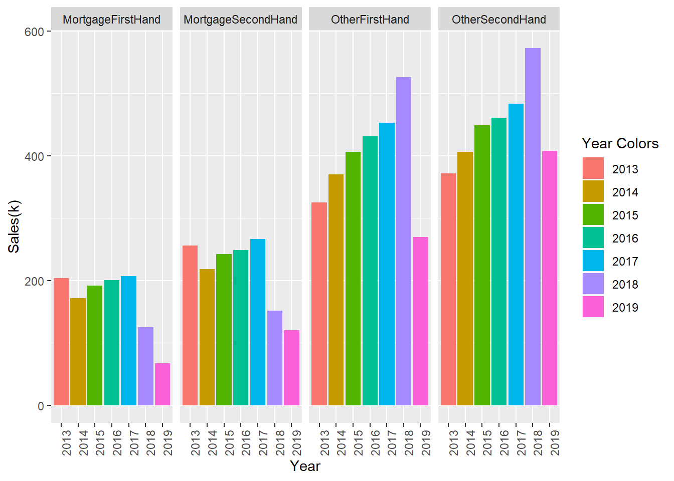

Total Sales Numbers through Years Comparising Five Big Cities with Population and the Others

df_hs_yearly_big_5_vs_others <- 
  sqldf ('select
  case when Province in ("Istanbul-34","Izmir-35","Ankara-6","Bursa-16","Antalya-7") then "Big_five"
    else "Others"
  end Big_Five_Flag, Year
  ,sum(Mortgaged_FirstHand_Sale) as MortgageFirstHand
  ,sum(Mortgaged_SecondHand_Sale) as MortgageSecondHand
  ,sum(Other_FirstHand_Sale) as OtherFirstHand
  ,sum(Other_SecondHand_Sale) as OtherSecondHand
from raw_data_province
group by case when Province in ("Istanbul-34","Izmir-35","Ankara-6","Bursa-16","Antalya-7")
  then "Big_five"
  else "Others"
  end, Year')

df_hs_yearly_big_5_pivot <- melt(df_hs_yearly_big_5_vs_others, id.vars = c("Year","Big_Five_Flag"),
                           measure.vars = c("MortgageFirstHand", "MortgageSecondHand","OtherFirstHand","OtherSecondHand" ))

ggplot(data = df_hs_yearly_big_5_pivot, aes(x = Year , y = value/1000 , group = Big_Five_Flag)) +
  #ggtitle("Plot of length \n by dose") + xlab("Dose (mg)") + ylab("Teeth length")
  geom_bar(aes(fill = factor(..x.., labels = "Year")), stat = "identity") +
  labs(fill = "Year") +
  facet_grid(~ Big_Five_Flag) +
  scale_y_continuous("Sales(k)") +
  theme(axis.text.x = element_text(angle = 90, hjust = 1))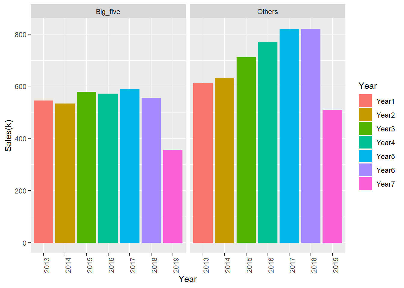

House Sales Numbers to Foreigners

House Sales to Foreigners covers the sales to the people that are defined as foreigner, non-Turkish originated and not subjected to law number 4112 in the database of General Directorate of Land Registry and Cadastre,“Turkey’s National Geographic Information System” (TUCBS), people that.

House sales numbers to foreigners data covered the first 10 city have been published since 2014.

Column names are below:

Year
Province
January
February
March
April
May
June
July
August
September
October
November
December

Provinces Covered by the Data

city=c("Istanbul","Antalya","Ankara","Bursa","Yalova","Sakarya","Trabzon","Mugla","Mersin","Aydin",
"Samsun","Izmir")
 
sett=sample(seq(0,1,0.01) , length(city) , replace=TRUE) 
 
par(bg="lightblue") 
wordcloud(city , sett , col=terrain.colors(length(city) , alpha=0.8) , rot.per=0.4 )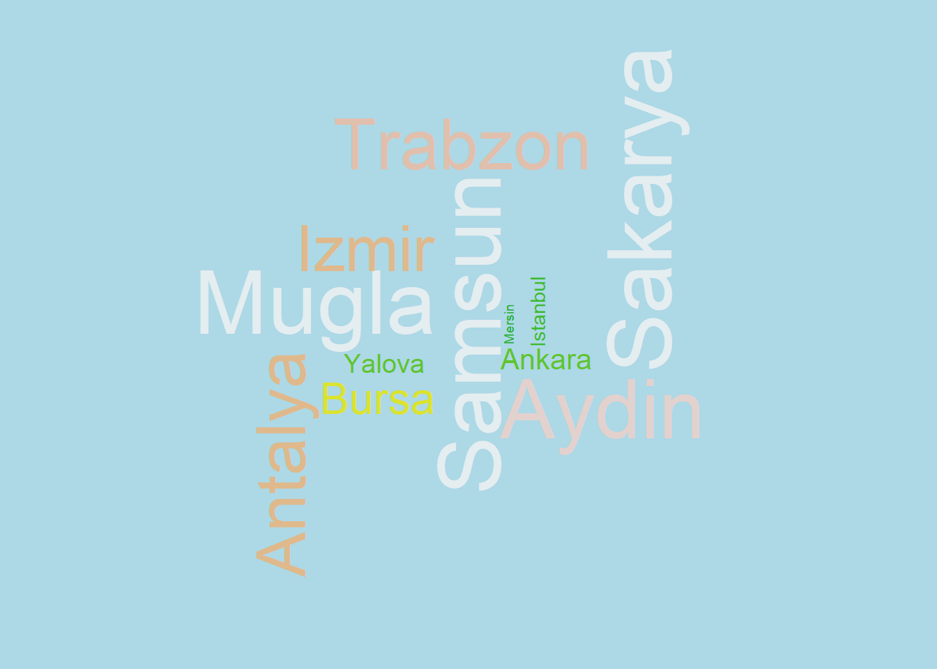

Provinces with the Highest Sales by Seasons

Tuik_Foreigners_sum<- Tuik_Foreigners %>% group_by(Province) %>% summarise(total_sum=sum(June+July+August),total_win=sum(December+January+February),total_sp=sum(March+April+May),total_aut=sum(September + October+ November )) %>% arrange(desc(total_sum))%>% mutate(
   rank =row_number(),vars_group = 'Province'
  ) %>% filter( Province!="Other provinces")


par(mfrow=c(2,2))


barplot(Tuik_Foreigners_sum$total_sp, las = 2, names.arg = Tuik_Foreigners_sum$Province,
        col ="pink", main ="Spring",
        ylab = "House Sales")

barplot(Tuik_Foreigners_sum$total_sum, las = 2, names.arg = Tuik_Foreigners_sum$Province,
        col ="yellow", main ="Summer",
        ylab = "House Sales")


barplot(Tuik_Foreigners_sum$total_sp, las = 2, names.arg = Tuik_Foreigners_sum$Province,
        col ="orange", main ="Autumn",
        ylab = "House Sales")


barplot(Tuik_Foreigners_sum$total_win, las = 2, names.arg = Tuik_Foreigners_sum$Province,
        col ="lightblue", main ="Winter",
        ylab = "House Sales")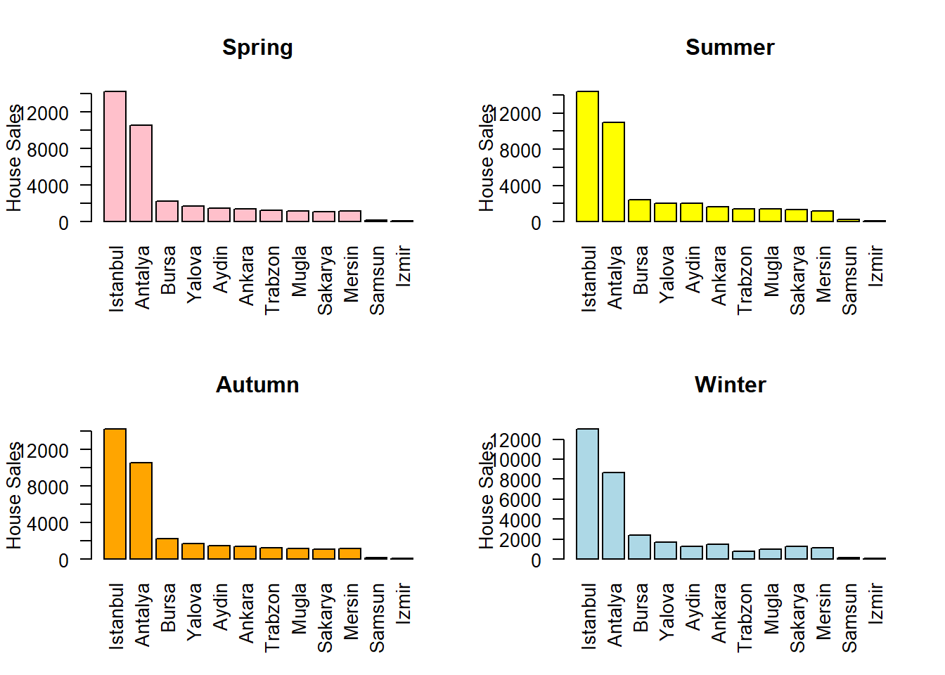

This plot states that seasons doesn’t have significant impact on house sales.

House Sales by Year

Tuik_Foreigners_by_year<- Tuik_Foreigners%>%filter( Province!="Other provinces") %>% group_by(Year) %>% summarise(total=sum(June+July+August+December+January+February+March+April+May+September + October+ November)) %>% arrange(Year) 


p1 <- ggplot() +
  geom_line(aes(y = total, x = Year), size=1.5, data = Tuik_Foreigners_by_year,
            stat="identity") +
  theme(legend.position="bottom", legend.direction="horizontal",
        legend.title = element_blank()) +
  scale_x_continuous(breaks=seq(2013,2019,1)) +
  labs(x="Year", y="House Sales") +
  ggtitle("Total of House Sales by Year") +
  theme(axis.line = element_line(size=1, colour = "black"), panel.grid.major = element_blank(),
        panel.grid.minor = element_blank(), panel.border = element_blank(),
        panel.background = element_blank()) +
  theme(plot.title=element_text(family="xkcd-Regular"), text=element_text(family="xkcd-Regular"),
        axis.text.x=element_text(colour="black", size = 10))
p1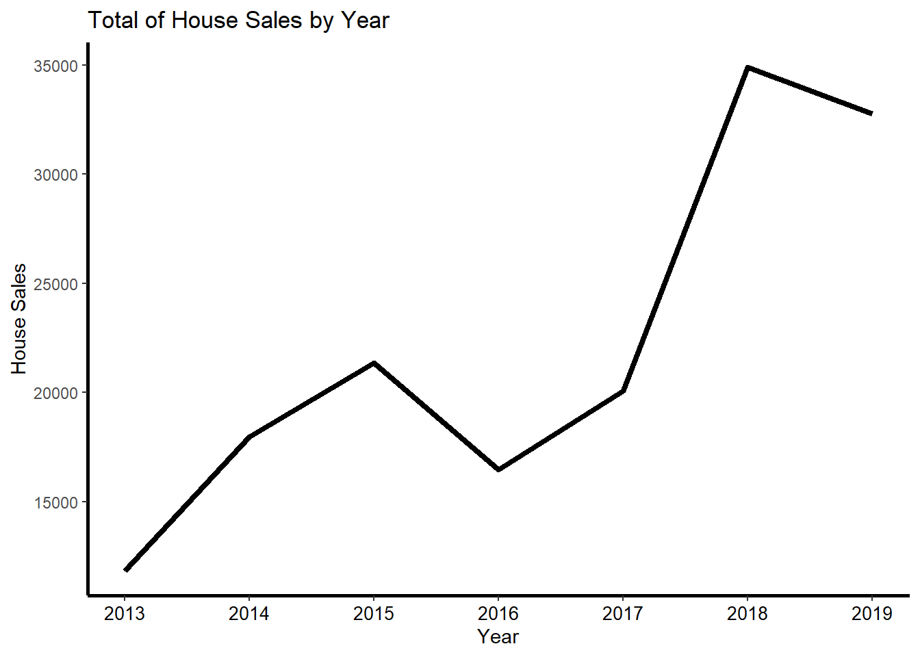

House sales to foreigners between 2017 and 2018 is remarkable increased. Since 2019 November and December sales could not be reflected into this analysis, the change between 2018 and 2019 could not be determined.

Turkey Sales Concentration Map

# Extract Turkey map data
TURKEY <- readRDS(url("https://github.com/pjournal/mef03g-road-runner/blob/master/TUIK-DATA/gadm36_TUR_1_sp.rds?raw=true"))
 
TURKEY@data %>% as_tibble() %>% head(10)

## # A tibble: 10 x 10
##    GID_0 NAME_0 GID_1 NAME_1 VARNAME_1 NL_NAME_1 TYPE_1 ENGTYPE_1 CC_1 
##    <chr> <chr>  <chr> <chr>  <chr>     <chr>     <chr>  <chr>     <chr>
##  1 TUR   Turkey TUR.~ Adana  Seyhan    <NA>      Il     Province  <NA> 
##  2 TUR   Turkey TUR.~ Adiya~ Adiyaman  <NA>      Il     Province  <NA> 
##  3 TUR   Turkey TUR.~ Afyon  Afyonkar~ <NA>      Il     Province  <NA> 
##  4 TUR   Turkey TUR.~ Agri   Agri|Kar~ <NA>      Il     Province  <NA> 
##  5 TUR   Turkey TUR.~ Aksar~ <NA>      <NA>      Il     Province  <NA> 
##  6 TUR   Turkey TUR.~ Amasya <NA>      <NA>      Il     Province  <NA> 
##  7 TUR   Turkey TUR.~ Ankara Ancara|A~ <NA>      Il     Province  <NA> 
##  8 TUR   Turkey TUR.~ Antal~ Adalia|A~ <NA>      Il     Province  <NA> 
##  9 TUR   Turkey TUR.~ Ardah~ <NA>      <NA>      Il     Province  <NA> 
## 10 TUR   Turkey TUR.~ Artvin Çoruh     <NA>      Il     Province  <NA> 
## # ... with 1 more variable: HASC_1 <chr>

TUR_for <- fortify(TURKEY)

## Regions defined for each Polygons

foreign_full<- Tuik_Foreigners  %>% select(Year,Province,Sales_Numbers)

Tuik_Foreigners_by_province<- Tuik_Foreigners%>%filter( Province!="Other provinces") %>% group_by(Province) %>% summarise(total=sum(June+July+August+December+January+February+March+April+May+September + October+ November)) %>% arrange(desc(total)) 

id_and_cities_full <- data_frame(id = rownames(TURKEY@data),
                            Province = TURKEY@data$NAME_1) %>% 
  left_join(Tuik_Foreigners_by_province, by = "Province")

final_map <- left_join(TUR_for, id_and_cities_full, by = "id")

head(final_map,10)

##        long      lat order  hole piece id group Province total
## 1  35.41454 36.58850     1 FALSE     1  1   1.1    Adana    NA
## 2  35.41459 36.58820     2 FALSE     1  1   1.1    Adana    NA
## 3  35.41434 36.58820     3 FALSE     1  1   1.1    Adana    NA
## 4  35.41347 36.58820     4 FALSE     1  1   1.1    Adana    NA
## 5  35.41347 36.58792     5 FALSE     1  1   1.1    Adana    NA
## 6  35.41236 36.58792     6 FALSE     1  1   1.1    Adana    NA
## 7  35.41236 36.58764     7 FALSE     1  1   1.1    Adana    NA
## 8  35.41208 36.58764     8 FALSE     1  1   1.1    Adana    NA
## 9  35.41208 36.58736     9 FALSE     1  1   1.1    Adana    NA
## 10 35.41180 36.58736    10 FALSE     1  1   1.1    Adana    NA

ggplot(final_map) +
  geom_polygon( aes(x = long, y = lat, group = group, fill = total),
                color = "grey") +
  coord_map() +
  theme_void() + 
  labs(title = "House Sales Numbers to Foreigners",
       subtitle = paste0("Total Sales Numbers of Houses: ",sum(Tuik_Foreigners_by_province$total)),
       caption = "Source: Türkiye İstatistik Kurumu") +
  scale_fill_distiller(name = "House Sales Numbers",
                       palette = "Spectral", limits = c(0,61000), na.value = "black") +
  theme(plot.title = element_text(hjust = 0.5),
        plot.subtitle = element_text(hjust = 0.5))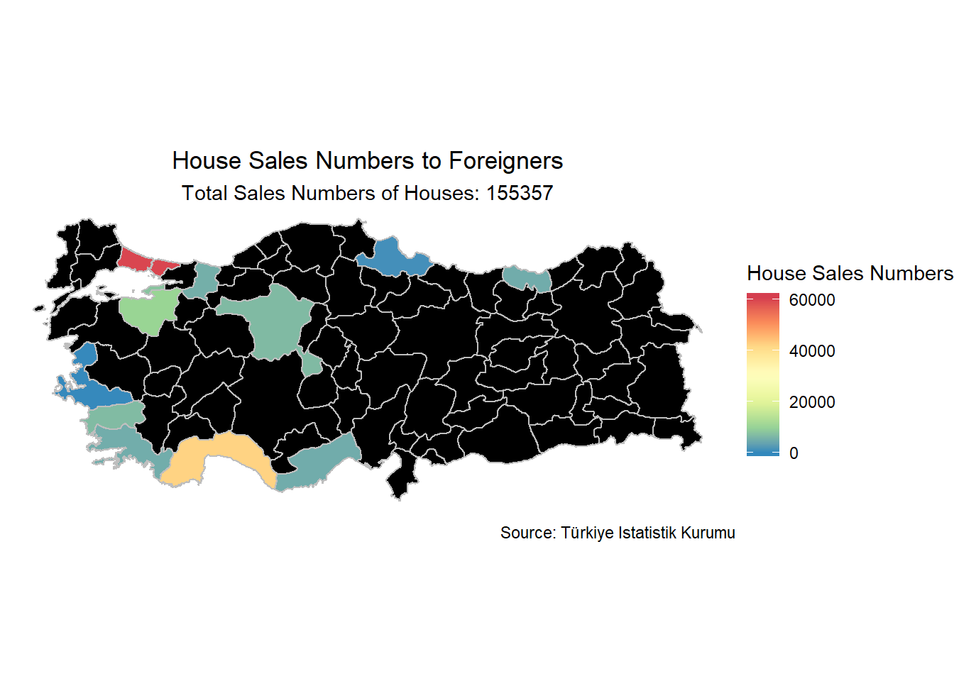

Istanbul has the highest sales density while Antalya follows. Although Samsun and Izmir have the lowest sales density

Total Sales Numbers to Foreigners with cities

House Sales Numbers in Detail of Genders in Turkey

House sales bumbers in detail of genders in Turkey covers the house sales in Turkey by men,women,common which indicates that a house is bought jointly by one or more than one woman and man and other refers to the house sales (corporate and foreign) other than those done by women and men individually or jointly.

Column names are below:

Year
City
Male
Female
Common
Other
Total

House Sales to men and women from 2014 to 2018

# Calculating house sales to males and females through years
yearly <-
raw_data_gender %>% 
  filter(City == 'Turkiye') %>%
  group_by(Year) %>%
  summarise(Women = sum(Female), Men = sum(Male)) %>%
  gather(Gender,Sales,-Year)

yearly

## # A tibble: 10 x 3
##     Year Gender  Sales
##    <int> <chr>   <int>
##  1  2014 Women  343209
##  2  2015 Women  382237
##  3  2016 Women  391334
##  4  2017 Women  409453
##  5  2018 Women  421286
##  6  2014 Men    695727
##  7  2015 Men    774874
##  8  2016 Men    801048
##  9  2017 Men    837928
## 10  2018 Men    790006

ggplot(yearly, aes(Year, Sales, group = Gender, color = Gender)) + geom_line() + geom_point() +
  scale_y_continuous(labels = comma)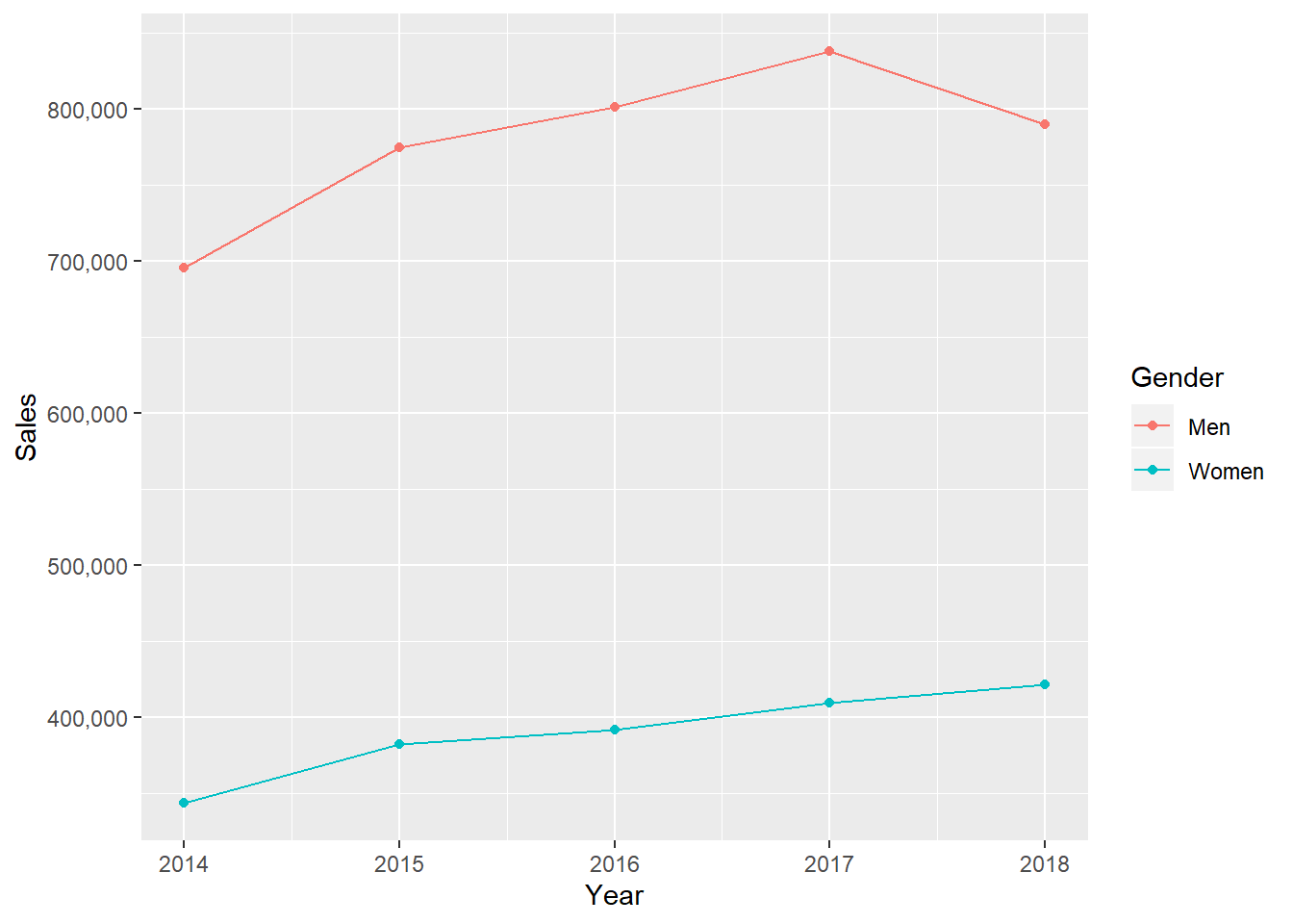

An interesting point here is, house sales to males from 2017 through 2018 is decreasing, altough sales to female in same period is increasing.

Cities has Highest Woman House Owners Ratio

top5_female <-
  raw_data_gender %>%
  group_by(City) %>%
  filter(City != "Türkiye") %>%
  summarise(Men = sum(Male), Women = sum(Female), Total = sum(Total)) %>%
  mutate(ratio = (Women / Total) * 100) %>%
  arrange(desc(ratio)) %>%
  mutate(rwn = row_number()) %>%
  filter(rwn < 6)

top5_female

## # A tibble: 5 x 6
##   City         Men  Women  Total ratio   rwn
##   <fct>      <int>  <int>  <int> <dbl> <int>
## 1 Balikesir  71843  52056 134427  38.7     1
## 2 Canakkale  33560  22861  62412  36.6     2
## 3 Mugla      43275  31173  87814  35.5     3
## 4 Edirne     19814  12617  35664  35.4     4
## 5 Izmir     211136 138118 390747  35.3     5

ggplot(top5_female, aes(x=City, y=ratio, fill=City))+
  geom_bar(stat="identity")+
  geom_text(aes(label = paste("%",round(ratio,3))), hjust=1.1, size=3.2)+
  coord_flip() +
  theme_minimal()+
  labs(x="City",y="Percentage",title="5 Cities has Highest Woman House Owners Ratio",fill="City")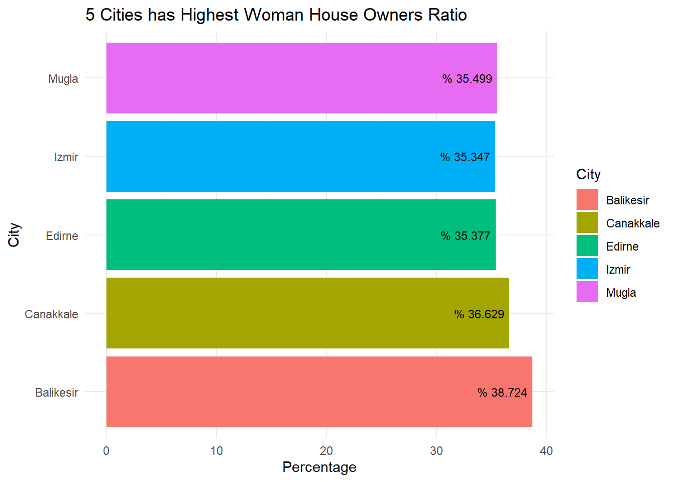

Balıkesir take the lead for female owners ratio among other cities while Canakkale follows. Ege, Marmara and Akdeniz are the regions has highest female house owner ratio.